Oct 10, 2016

SG Series Part 6: Step Into The Baking Lab

bakinglab_post_intro

This is part 6 of a series on Spherical Gaussians and their applications for pre-computed lighting. You can find the other articles here:

Part 1 - A Brief (and Incomplete) History of Baked Lighting Representations
Part 2 - Spherical Gaussians 101
Part 3 - Diffuse Lighting From an SG Light Source
Part 4 - Specular Lighting From an SG Light Source
Part 5 - Approximating Radiance and Irradiance With SG’s
Part 6 - Step Into The Baking Lab

Get the code on GitHub: https://github.com/TheRealMJP/BakingLab (pre-compiled binaries available here)

Back in early 2014, myself and David Neubelt started doing serious research into using Spherical Gaussians as a compact representation for our pre-computed lighting probes. One of the first things I did back then was to create a testbed application that we could use to compare various lightmap representations (SH, H-basis, SG, etc.) and quickly experiment with new ideas. As part of that application I implemented my first path tracer, which was directly integrated into the app for A/B comparisons. This turned out to be extremely useful, since having quick feedback was really helpful for evaluating quality and also for finding and fixing bugs. Eventually we used this app to finalize the exact approach that we would use when integrating SG’s into The Order: 1886.

A year later in 2015, Dave and I created another test application for experimenting with improvements that we were planning for future projects. This included things like a physically based exposure model utilizing real-world camera parameters, using the ACES[1] RRT/ODT for tone mapping, and using real-world units[2] for specifying lighting intensities. At some point I integrated an improved version of SG baking into this app that would progressively compute results in the background while the app remained responsive, allowing for quick “preview-quality” feedback after adjusting the lighting parameters. Once we started working on our SIGGRAPH presentation[3] from the 2015 physically based shading course, it occurred to us that we should really package up this new testbed and release it alongside the presentation to serve as a working implementation of the concepts we were going to cover. But unfortunately this slipped through the cracks: the new testbed required a lot of work in order to make it useful, and both Dave and I were really pressed for time due to multiple new projects ramping up at the office.

Now, more than a year after our SIGGRAPH presentation, I’m happy to announce that we’ve finally produced and published a working code sample that demonstrates baking of Spherical Gaussian lightmaps! This new app, which I call “The Baking Lab”, is essentially a combination of the two testbed applications that we created. It includes all of the fun features that we were researching in 2015, but also includes real-time progressive baking of 2D lightmaps in various formats. It also allows switching to a progressive path tracer at any time, which serves as the “ground truth” for evaluating lightmap quality and accuracy. Since it’s an amalgamation of two older apps, it uses D3D11 and the older version of my sample framework. So there’s no D3D12 fanciness, but it will run on Windows 7. If you’re just interested in looking at the code or running the app, then go ahead and head over to GitHub: https://github.com/TheRealMJP/BakingLab. If you’re interested in the details of what’s implemented in the app, then keep reading.

Lightmap Baking

The primary feature of The Baking Lab is lightmap baking. Each of the test scenes includes a secondary UV set that contains non-overlapping UV’s used for mapping the lightmap onto the scene. Whenever the app starts or a new scene is selected, the baker uses the GPU to rasterize the scene into lightmap UV space. The pixel shader outputs interpolated vertex components like position, tangent frame, and UV’s to several render targets, which use MSAA to simulate conservative rasterization. Once the rasterization is completed, the results are copied back into CPU-accessible memory. The CPU then scans the render targets, and extracts “bake points” from all texels covered by the scene geometry. Each of these bake points represents the location of a single hemispherical probe to be baked.

Once all bake points are extracted, the baker begins running using a set of background threads on the CPU. Each thread continuously grabs a new work unit consisting of a group of contiguous bake points, and then loops over the bake points to compute the result for that probe. Each probe is computed by invoking a path tracer, which uses Embree[4] to allow for arbitrary ray tracing through the scene on the CPU. The path tracer returns the incoming radiance for a direction and starting point, where the radiance is the result of indirect lighting from various light sources as well as the direct lighting from the sky. The path tracer itself is a very simple unidirectional path tracer, using a few standard techniques like importance sampling, correlated multi-jittered sampling[5], and russian roulette to increase performance and/or convergence rates. The following baking modes are supported:

Diffuse - a single RGB value containing the result of applying a standard diffuse BRDF to the incoming lighting, with an albedo of 1.0
Half-Life 2 - directional irradiance projected onto the Half-Life 2 basis[6], making for a total of 3 sets of RGB coefficients (9 floats total)
L1 SH - radiance projected onto the first two orders of spherical harmonics, making for a total of 4 sets of RGB coefficients (12 floats total). Supports environment specular via a 3D lookup texture.
L2 SH - radiance projected on the first three orders of spherical harmonics, making for a total of 9 sets of RGB coefficients (27 floats total). Supports environment specular via a 3D lookup texture.
L1 H-basis - irradiance projected onto the first two orders of H-basis[7], making for a total of 4 sets of RGB coefficients (12 floats total).
L2 H-basis - irradiance projected onto the first three orders of H-basis, making for a total of 6 sets of RGB coefficients (18 floats total).
SG5 - radiance represented by the sum of 5 SG lobes with fixed directions and sharpness, making for a total of 5 sets of RGB coefficients (15 floats total). Supports environment specular via an approximate evaluation of per-lobe specular contribution.
SG6 - radiance represented by the sum of 6 SG lobes with fixed directions and sharpness, making for a total of 6 sets of RGB coefficients (18 floats total). Supports environment specular via an approximate evaluation of per-lobe specular contribution.
SG9 - radiance represented by the sum of 9 SG lobes with fixed directions and sharpness, making for a total of 9 sets of RGB coefficients (27 floats total). Supports environment specular via an approximate evaluation of per-lobe specular contribution.
SG12 - radiance represented by the sum of 12 SG lobes with fixed directions and sharpness, making for a total of 12 sets of RGB coefficients (36 floats total). Supports environment specular via an approximate evaluation of per-lobe specular contribution.

For SH, H-basis, and HL2 basis baking modes the path tracer is evaluated for random rays distributed about the hemisphere so that Monte Carlo integration can be used to integrate the radiance samples onto the corresponding basis functions. This allows for true progressive integration, where the baker makes N passes over each bake point, each time adding a new sample with the appropriate weighting. It looks pretty cool in action:

The same approach is used for the “Diffuse” baking mode, except that sampling rays are evaluated using a cosine-weighted hemispherical sampling scheme[8]. For SG baking, things get a little bit trickier. If the ad-hoc projection mode is selected, the result can be progressively evaluated in the same manner as the non-SG bake modes. However if either the Least Squares or Non-Negative Least Squares mode are active, we can’t run the solve unless we have all of the hemispherical radiance samples available to feed to the solver. In this case we switch to a different baking scheme where each thread fully computes the final value for every bake point that it operates on. However the thread only does this for a single bake point from each work group, and afterwards it fills in the rest of the neighboring bake points (which are arranged in a 8x8 group of texels) with the results it just computed. Each pass of of baker then fills in the next bake point in the work group, gradually computing the final result for all texels in the group. So instead of seeing the quality slowly improve across the light map, you see extrapolated results being filled in. It ends up looking like this:

While it’s not as great as a true progressive bake, it’s still better than having no preview at all.

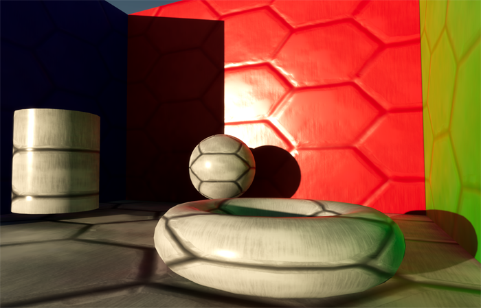
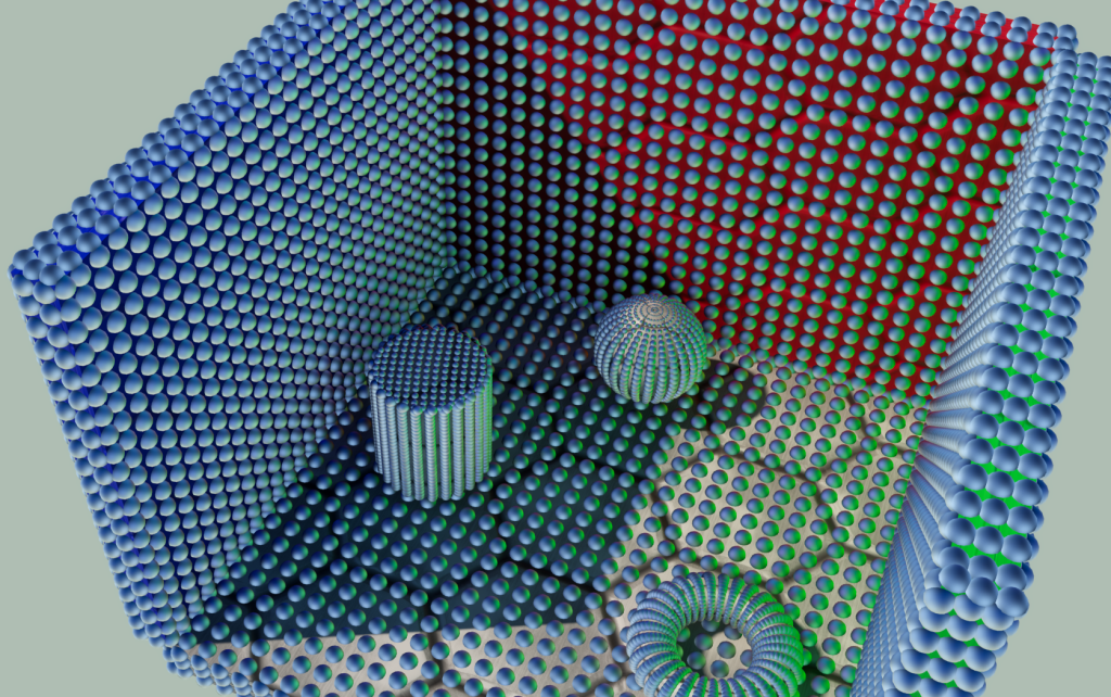
The app supports a few settings that control some of the bake parameters, such as the number of samples evaluated per-texel and the overall lightmap resolution. The “Scene” group in the UI also has a few settings that allow toggling different components of the final render, such as the direct or indirect lighting or the diffuse/specular components. Under the “Debug” setting you can also toggle a neat visualizer that shows a visual representation of the raw data stored in the lightmap. It looks like this:

SG_Debug_Visualizer

Ground Truth Path Tracer

The integrated path tracer is primarily there so that you can see how close or far off you are when computing environment diffuse or specular from a light map. It was also a lot of fun to write - I recommend doing it sometime if you haven’t already! Just be careful: it may make you depressed to see how poorly your real-time approximation holds up when compared with a proper offline render. :-)

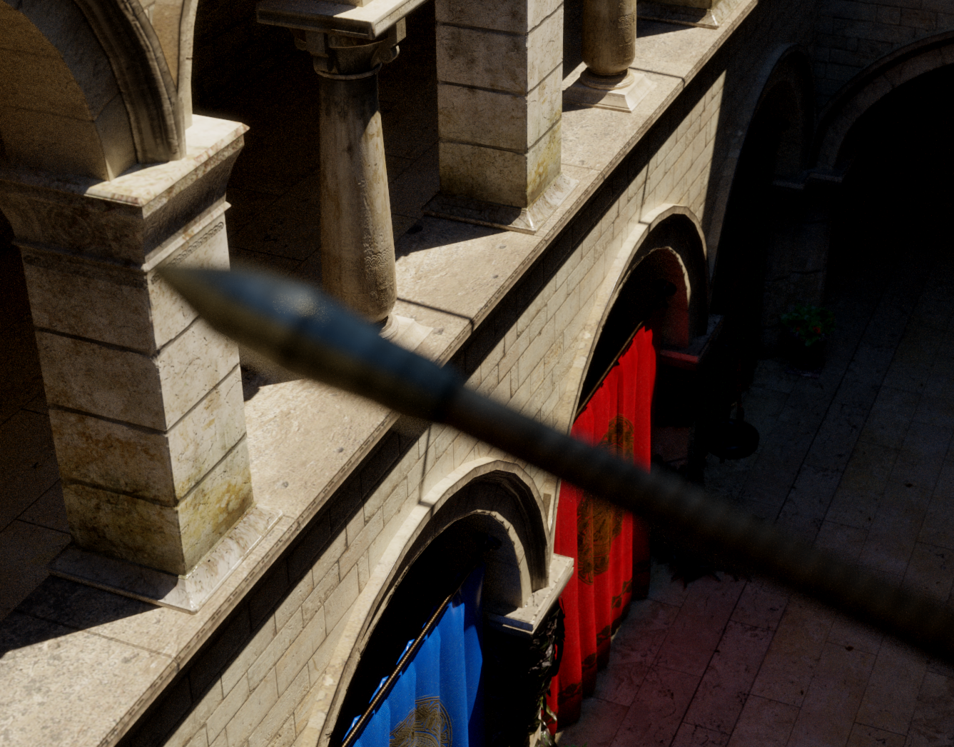
The ground truth renderer works in a similar vein to the lightmap baker: it kicks off multiple background threads that each grab work groups of 16x16 pixels that are contiguous in screen space. The renderer makes N passes over each pixel, where each pass adds an additional sample that’s weighted and summed with the previous results. This gives you a true progressive render, where the result starts out noisy and (very) gradually converges towards a noise-free image:

The ground truth renderer is activated by checking the “Show Ground Truth” setting under the “Ground Truth” group. There’s a few more parameters in that group to control the behavior of the renderer, such as the number of samples used per-pixel and the scheme used for generating random samples.

Light Sources

There’s 3 different light sources supported in the app: a sun, a sky, and a spherical area light. For real-time rendering, the sun is handled as a directional light with an intensity computed automatically using the Hosek-Wilkie solar radiance model[9]. So as you change the position of the sun in the sky, you’ll see the color and intensity of the sunlight automatically change. To improve the real-time appearance, I used the disk area light approximation from the 2014 Frostbite presentation. The path tracer evaluates the sun as an infinitely-distant spherical area light with the appropriate angular radius, with uniform intensity and color also computed from the solar radiance model. Since the path tracer handles the sun as a true area light source, it produces correct specular reflections and soft shadows. In both cases the sun defaults to correct real-world intensities using actual photometric units. There is a parameter for adjusting the sun size, which will result in the sun being too bright or too dark if manipulated. However there’s another setting called “Normalize Sun Intensity” which will attempt to maintain roughly the same illumination regardless of the size, which allows for changing the sun appearance or shadow softness without changing the overall scene lighting.

The default sky mode (called “Procedural”) uses the Hosek-Wilkie sky model to compute a procedural sky from a few input parameters. These include turbidity, ground albedo, and the current sun position. Whenever the parameters are changed, the model is cached to a cubemap that’ s used for real-time rendering on the GPU. For CPU path tracing, the the sky model is directly evaluated for a direction using the sample code provided by the authors. When combined with the procedural sun model, the two light sources form a simple outdoor lighting environment that corresponds to real-world intensities. Several other sky modes are also supported for convenience. The “Simple"mode takes just a color and intensity as input parameter, and flood-fills the entire sky with a value equal to color * intensity. The “Ennis”, “Grace Cathedral”, and “Uffizi Cross” modes use corresponding HDR environment maps to fill the sky instead of a procedural model.

For local lighting, the app supports enabling a single spherical area light using the “Enable Area Light” setting. The area light can be positioned using the Position X/Position Y/Position Z settings, and its radius can be specified with the “Size” setting. There are a 4 different modes for specifying the intensity of the light:

Luminance - the intensity corresponds to the amount of light being emitted from the light source along an infinitesimally small ray towards the viewer or receiving surface. Uses units of cd/m2. Changing the size of the light source will change the overall illumination the scene.
Illuminance - specifies the amount of light incident on a surface at a set distance, which is specified using the “Illuminance Distance” setting. So instead of saying “how much light is coming out of the light source” like you do with the “Luminance” mode, you’re saying “how much diffuse light is being reflected from a perpendicular surface N units away”. Uses units of lux, which are equivalent to lm/m2. Changing the size of the light source will not change the overall illumination the scene.
Luminous Power - specifies the total amount of light being emitted from the light source in all directions. Uses units of lumens. Changing the size of the light source will not change the overall illumination the scene.
EV100 - this is an alternative way of specifying the luminance of the light source, using the exposure value[10] system originally suggested by Nathan Reed[11]. The base-2 logarithmic scale for this mode is really nice, since incrementing by 1 means doubling the perceived brightness. Changing the size of the light source will change the overall illumination the scene.

The ground truth renderer will evaluate the area light as a true spherical light source, using importance sampling to reduce variance. The real-time renderer approximates the light source as a single SG, and generates very simple hard shadows using an array of 6 shadow maps. By default only indirect lighting from the area light will be baked into the lightmap, with the direct lighting evaluated on the GPU. However if the “Bake Direct Area Light” setting is enabled, then the direct contribution from the area light will be baked into the lightmap.

Note that all light sources in the app are always scaled down by a factor of 2-10 before being using in rendering, as suggested by Nathan Reed in his blog post[11]. Doing this effectively shifts the window of values that can be represented in a 16-bit floating point value, which is necessary in order to represent specular reflections from the sun. However the UI always will always show the unshifted values, as will the debug luminance picker that shows the final color and intensity of any pixel on the screen.

Exposure and Depth of Field

As I mentioned earlier, the app implements a physically based exposure system that attempts to models the behavior and parameters of a real-world camera. Much of the implementation was based on the code from Padraic Hennessy’s excellent series of articles[12], which was in turn inspired by Sébastien Lagarde and Charles de Rousiers’s SIGGRAPH presentation from 2014[2]. When the “Exposure Mode” setting is set to the “Manual (SBS)” or “Manual (SOS)” modes, the final exposure value applied before tone mapping will be computed based on the combination of aperture size, ISO rating, and shutter speed. There is also a “Manual (Simple)” mode available where a single value on a log2 scale can be used instead of the 3 camera parameters.

Mostly for fun, I integrated a post-process depth of field effect that uses the same camera parameters (along with focal length and film size) to compute per-pixel circle of confusion sizes. The effect is off by default, and can be toggled on using the “Enable DOF” setting. Polygonal and circular bokeh shapes are supported using the technique suggested by Tiago Sousa in his 2013 SIGGRAPH presentation[13]. Depth of field is also implemented in the ground truth renderer, which is capable of achieving true multi-layer effects by virtue of using a ray tracer.

Tone Mapping

Several tone mapping operators are available for experimentation:

Linear - no tone mapping, just a clamp to [0, 1]
Film Stock - Jim Hejl and Richard Burgess-Dawson’s polyomial approximation of Haarm-Peter Duiker’s filmic curve, which was created by scanning actual film stock. Based on the implementation provided by John Hable[14].
Hable (Uncharted2) - John Hable’s adjustable filmic curve from his GDC 2010 presentation[15]
Hejl 2015 - Jim Hejl’s filmic curve that he posted on Twitter[16], which is a refinement of Duiker’s curve
ACES sRGB Monitor - a fitted polynomial version of the ACES[17] reference rendering transform (RRT) combined with the sRGB monitor output display transform (ODT), generously provided by Stephen Hill.

Debug Settings

At the bottom of the settings UI are a group of debug options that can be selected. I already mentioned the bake data visualizer previously, but it’s worth mentioning again because it’s really cool. There’s also a “luminance picker”, which will enable a text output showing you the luminance and illuminance of the surface under the mouse cursor. This was handy for validating the physically based sun and sky model, since I could use the picker to make sure that the lighting values matched what you would expect from real-world conditions. The “View Indirect Specular” option causes both the real-time renderer and the ground truth renderer to only show the indirect specular component, which can be useful for gauging the accuracy of specular computed from the lightmap. After that there’s a pair of buttons for saving or loading light settings. This will serialize the settings that control the lighting environment (sun direction, sky mode, area light position, etc.) to a file, which can be loaded in whenever you like. The “Save EXR Screenshot” is fairly self-explanatory: it lets you save a screenshot to an EXR file that retains the HDR data. Finally there’s an option to show the current sun intensity that’s used for the real-time directional light.

References

[1] Academy Color Encoding System
[2] Moving Frostbite to PBR (course notes)
[3] Advanced Lighting R&D at Ready At Dawn Studios
[4] Embree: High Performance Ray Tracing Kernels
[5] Correlated Multi-Jittered Sampling
[6] Shading in Valve’s Source Engine
[7] Efficient Irradiance Normal Mapping
[8] Better Sampling
[9] Adding a Solar Radiance Function to the Hosek Skylight Model
[10] Exposure value
[11] Artist-Friendly HDR With Exposure Values
[12] Implementing a Physically Based Camera: Understanding Exposure
[13] CryENGINE 3 Graphics Gems
[14] Filmic Tonemapping Operators
[15] Uncharted 2: HDR Lighting
[16] Jim Hejl on Twitter
[17] Academy Color Encoding System Developer Resources

Comments:

dev - Jan 2, 2019

thanks for the great article, sorry about the beginner question but I wanted to know if there are some considerations we need to know if we want to add more lights to the scene,

#### [MJP](http://mynameismjp.wordpress.com/ "mpettineo@gmail.com") - Jun 0, 2017

Does your FBX file have a secondary UV set? The demo requires that the scene have a second UV set that has a unique UV parameterization for the whole scene, since it uses it for the generated lightmap.

#### []( "") - Aug 3, 2018

Hello, Thanks for providing the baking lab source code and these articles! Does the baking lab contain any sample code for how one could have a dynamic mesh lit from the lightmaps?

#### [MJP](http://mynameismjp.wordpress.com/ "mpettineo@gmail.com") - Aug 3, 2018

Unfortunately it does not: it only shows how to bake 2D lightmaps for suitable static geometry. Each texel of the lightmap bakes the incoming lighting for a hemisphere surrounding the surface normal of the mesh, which means that the information is only useful if being applied to that particular surface. For dynamic meshes, you typically want to bake a set of spherical probes (containing lighting from all directions, and not just on a hemisphere) throughout the entire area that your meshes might be moving. A simple way to do this is to place all of probes within cells of a 3D grid that surrounds your scene, which makes it simple to figure out which probe(s) to sample from, and also makes it simple to interpolate between neighboring probes. It’s also possible to use less regular representations that are more sparse in areas with less lighting/geometry complexity, or that rely on hand-placed probes. This can save you memory and/or baking time, but can make probe lookups and interpolation more costly. Either way baking the probe itself is very similar to the code in the sample for baking a hemisphere, with the major difference being that you need to shoot rays in all directions and adjust your monte carlo weights accordingly. You also have to choose a basis that can represent lighting on a sphere, for instance spherical harmonics or a set of SG’s oriented about the unit sphere. Part 5 of the article talks a bit about working with these representations, and the tradeoffs involved.

#### [MJP](http://mynameismjp.wordpress.com/ "mpettineo@gmail.com") - Mar 0, 2017

Hi Steven, Sorry that I took so long to reply to your question. The answer here is “yes”, since samples at the extreme edges of the hemisphere can potentially result in a negative contribution when projected onto the basis vectors. HL2 basis is exactly like spherical harmonics in this regard, except that the way the basis vectors are oriented results in ideal projections for a hemisphere since each basis vector has the same projection onto the local Z axis (normal) of the baking point. In fact, HL2 is pretty much exactly the same as L1 SH, except it has different weighting and the basis vectors are rotated (in SH the linear cosine lobes are lined up with the major X/Y/Z axes). This is actually noted in Habel’s paper from 2010 where they introduce H-basis: https://www.cg.tuwien.ac.at/research/publications/2010/Habel-2010-EIN/Habel-2010-EIN-paper.pdf (see section 2.1)

#### [Steven]( "steven.brekelmans@gmail.com") - Feb 6, 2017

First of all thank you for the great series. I have a question about the HL2Baker - when the sample is projected onto the three basis vectors in AddSample(), there’s no clamp for rejecting samples that point *away* from the basis. Doesn’t this effectively remove power from the accumulation for that basis since the dot product would be negative?

#### [MJP](http://mynameismjp.wordpress.com/ "mpettineo@gmail.com") - Oct 0, 2016

Hey Max, I’m glad you enjoyed the articles! The incorrect luminance calculation was an oversight on my part. I must have copy-pasted the formula from some older code without double-checking that I was using the correct weights for computing relative luminance from linear sRGB values. I’ve corrected the code in that shader, and also fixed a few other places where I was using the incorrect formula. Thank you for pointing that out!

#### [Rim]( "remigius@netforge.nl") - Oct 3, 2016

Great stuff as always Matt, posts like this make me want to do 3D graphics again :)

#### [MJP](http://mynameismjp.wordpress.com/ "mpettineo@gmail.com") - Oct 4, 2016

Thank you Rim, nice to hear from you again! There’s always time for a little graphics on the side. ;)

#### [Max]( "msomeone@gmail.com") - Oct 6, 2016

Thank you for writing this awesome articles series and releasing BakingLab! I`m very curious why in illuminance computation in Mesh.hlsl shader there are 0.299f, 0.587f, 0.114f weight, not rec.709\sRGB relative luminance weights? Is it somehow related to usage of Hosek’s sky model?

#### [MJP](http://mynameismjp.wordpress.com/ "mpettineo@gmail.com") - Apr 4, 2017

Hey! So pretty much the entire pipeline works in the a space such that intensity is scaled down by the 2^-10 factor, with all inputs (environment maps, light sources) appropriately scaled down to match that space. This includes the average luminance calculation and exposure calculations. There’s no need to ever “restore” back to the physical intensity range, since you get the correct final results by keeping the scene radiance and exposure values in the same 2^-10 space. Does that make sense? Sorry that the code is a bit confusing when it comes to that scale factor, I probably should have added a few more comments explaining what was going on with that. -Matt

#### [olej]( "olejpoland@gmail.com") - Nov 6, 2016

Hey Matt, First of all thanks for all your hard work and sharing it with us :). Your contributions are invaluable to the graphics programming community. As some unfamiliar with offline rendering middlewares, I was wondering why use Embree for ground truth reference? I remember you mentioning that your bake farms on The Order used OptiX. I would guess that a GPU raytracer would converge way faster then a CPU one, especially when you are limited to a single machine. What are your reasons for this choice and what library would you recommend to someone wanting to write a reference GI preview for a game engine?

#### [User1]( "mendele@yandex.ru") - Apr 4, 2017

Hello MJP! Thanks for sharing. My question is regarding average luminance calculation. LuminanceReductionInitialCS takes as input a back buffer with luminance scaled down with 2^-10, and operates on that values without restoring actual luminance. But restoring gives wrong results (everything becomes too dark). What’s the logic behind that? Thanks.

#### [Sze](http://divrgents.com "awu.chen.dev@gmail.com") - Jun 3, 2017

Hi MJP, Thank you so much for providing this extensive blog and the source code. I am running into problems bringing in an external .fbx file into the project. I’ve tried modifying the Model filenames as well as creating an entirely new fbx file in the BakingLab.cpp however it’s giving me errors “block offset if out of range” or “DirectX Error: The parameter is incorrect” It will be amazing if you can let me know how I should proceed with bringing in external fbx files. Thanks again.

#### [MJP](http://mynameismjp.wordpress.com/ "mpettineo@gmail.com") - Nov 6, 2016

I haven’t seen any concrete numbers in a while, but I would imagine that OptiX on a high-end GPU will have higher throughput than running Embree on a high-end consumer CPU. However I find Embree much easier to work with, which is why I use it for non-work projects. The Embree API is very clean with few entrypoints, and it’s very simple to use it to build an acceleration structure from triangle meshes. From there you can just cast arbitrary rays however you’d like, which makes it very easy to fit into your renderer. I would also consider it to be pretty fast and well-optimized, even if it can’t match the throughput of a GPU-based ray tracer. The OptiX API is also nice, but it’s much more complex than Embree. This is becase OptiX isn’t just a ray-tracing kernel: it’s also a framework for writing a complete renderer. The framework is important because it abstracts away some of the details of CUDA and the underlying GPU architecture, which is inherently less flexible than pure CPU code. This allows you to write a ray-generation program that runs persistently while the GPU traces the rays and runs separate programs whenever a ray intersects a triangle. They also have an API that they call “OptiX Prime”, which is just the ray-tracing kernel. I haven’t used it myself, but I would imagine it might be tricky to use in a way that plays nicely with a GPU. Either way, if you use it then you’ve effectively restricted yourself to Nvidia hardware. At work we don’t care as much since we can just keep buying Nvidia GPU’s, but that’s not a great option for a public demo. At work we also run Linux on the bake farm PC’s, which helps avoid some annoying issues that can pop up when using CUDA on a Windows PC. However we’ve still had plenty of issues with drivers, overheating, running out of memory, and lack of debugging support. I think for your purposes Embree would be just fine. Like I just explained it’s much easier to integrate, especially when you consider that you can natively debug your code. If you want to make it as fast as you can then you can consider using ISPC to vectorize your code.You may also want to look into AMD’s FireRays, which can use Embree as a back-end or run on the GPU: http://gpuopen.com/firerays-2-0-open-sourcing-and-customizing-ray-tracing/ I haven’t looked at it myself, but I would imagine that the API is heavier than Embree’s due to the need to abstract away multiple back-ends.

#### [郭叉叉 (@guoxx_)](http://twitter.com/guoxx_ "guoxx_@twitter.example.com") - Jun 1, 2017

Amazing articles. Thanks for sharing those experience and source code. I have one question about the relative luminance calculation, the equation used is well described in BT.709 standard. But I think it’s working with radiometry unit. Since the luminance unit is used for light, relative luminance shouldn’t use another equation? For example, there is a light with color temperature and randiant power defined, we can construct a spectrum data and luminous efficiency base on color temperature, after photometric curve weighted, RGB value with photometry unit is used for lighitng, then luminance is stored in backbuffer. If we apply the equation from BT.709. does photometric curve applied twice since curve is already applied when we convert light units from radiometry to photometry? I think the correct way is luminance = r * integral_of_srgb_r_responce_curve + g * integral_of_srgb_g_responce_curve + b * integral_of_srgb_b_responce_curve Please point it out if I made any mistake.

#### [MJP](http://mynameismjp.wordpress.com/ "mpettineo@gmail.com") - Oct 2, 2016

Hey Stephen, thank you for the kind words! Yes, you could absolutely save off the “Lightmap” resource as a file and then re-load later. In fact there’s a helper function in Textures.h called “SaveTextureAsDDS” that you could use to do this, and it will save the save the entire texture array as a DDS file containing uncompressed fp16 data.

#### [Wumpf](http://wumpfblog.wordpress.com "r_andreas2@web.de") - Oct 6, 2016

Thank you so much for this article series! Haven’t done much graphics stuff for quite some time - all those cross references will keep me busy for a while :). I especially enjoyed how you’ve described the practical considerations of the production environment in Part 5. It must have been quite annoying to drop the accurate fitting algorithm for the (albeit creative) hack to make it run on a large scale within the time constraints.

#### [Stephen Keefer](https://www.facebook.com/app_scoped_user_id/10155402927081038/ "keefer.stephen@gmail.com") - Oct 2, 2016

Very nice article and description! Excellent sample application and makes me wanna incorporate this into my editor. I am curious about a few things Am I correct in assuming that, if you were to save “Lightmap” resource view from “MeshBakerStatus” after the progress reaches 100%, you could then reuse this in next launch (or in game), assuming light parameters are the same.