SG Series Part 2: Spherical Gaussians 101

This is part 2 of a series on Spherical Gaussians and their applications for pre-computed lighting. You can find the other articles here:

Part 1 - A Brief (and Incomplete) History of Baked Lighting Representations
Part 2 - Spherical Gaussians 101
Part 3 - Diffuse Lighting From an SG Light Source
Part 4 - Specular Lighting From an SG Light Source
Part 5 - Approximating Radiance and Irradiance With SG’s
Part 6 - Step Into The Baking Lab

In the previous article, I gave a quick rundown of some of the available techniques for representing a pre-computed distribution of radiance or irradiance for each lightmap texel or probe location. In this article, I’m going cover the basics of Spherical Gaussians, which are a type of spherical radial basis function (SRBF for short). The concepts introduced here will serve as the core set of tools for working with Spherical Gaussians, and in later articles I’ll demonstrate how you can use those tools to form an alternative for approximating incoming radiance in pre-computed lightmaps or probes.

I should point out that this article is still going to be somewhat high-level, in that it won’t provide full derivations and background details for all formulas and operations. However it is my hope that the material here will be sufficient to gain a basic understanding of SG’s, and also use them in practical scenarios.

What’s a Spherical Gaussian?

A Spherical Gaussian, or “SG” for short, is essentially a Gaussian function[1] that’s defined on the surface of a sphere. If you’re reading this, then you’re probably already familar with how a Gaussian function works in 1D: you compute the distance from the center of the Gaussian, and use this distance as part of a base-e exponential. This produces the characteristic “hump” that you see when you graph it:

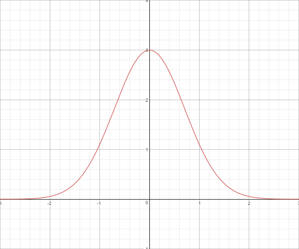
You’re probably also familiar with how it looks in 2D, since it’s very commonly used in image processing as a filter kernel. It ends up looking like what you would get if you took the above graph and revolved it around its axis

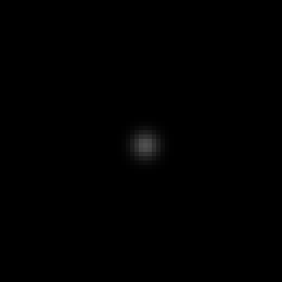
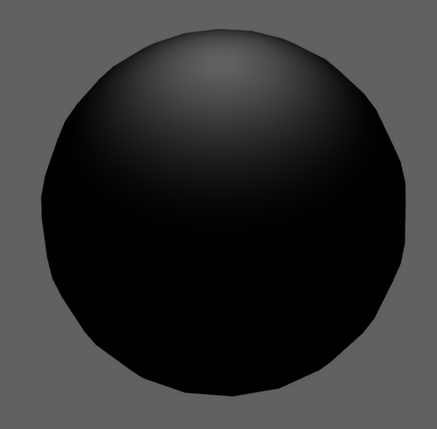
A Spherical Gaussian still works the same way, except that it now lives on the surface of a sphere instead of on a line or a flat plane. If you’re having trouble visualizing that, imagine if you took the above image and wrapped it around a sphere like wrapping paper. It ends up looking like this:

Since an SG is defined on a sphere rather than a line or plane, it’s parameterized differently than a normal Gaussian. A 1D Gaussian function always has the following form:

$$ ae^{\frac{-(x - b)^{2}}{2c^{2}}} $$

The part that we need to change in order to define the function on a sphere is the “(x - b)” term. This part of the function essentially makes the Gaussian a function of the cartesian distance between a given point and the center of the Gaussian, which can be trivially extended into 2D using the standard distance formula. To make this work on a sphere, we must instead make our Gaussian a function of the angle between two unit direction vectors. In practice we do this by making an SG a function of the cosine of the angle between two vectors, which can be efficiently computed using a dot product like so:

$$ G(\mathbf{v};\mathbf{\mu},\lambda,a) = ae^{\lambda(\mathbf{\mu} \cdot \mathbf{v} - 1)} $$

Just like a normal Gaussian, we have a few parameters that control the shape and location of the resulting lobe. First we have μ, which is the axis, or direction of the lobe. It effectively controls where the lobe is located on the sphere, and always points towards the exact center of the lobe. Next we have λ, which is the sharpness of the lobe. As this value increases, the lobe will get “skinnier”, meaning that the result will fall off more quickly as you get further from the lobe axis. Finally we have a, which is the amplitude or intensity of the lobe. If you were to look at a polar graph of an SG, it would correspond to the height of the lobe at its peak. The amplitude can be a scalar value, or for graphics applications we may choose to make it an RGB triplet in order to support varying intensities for different color channels. This all lends itself to a simple HLSL code definition:

struct SG
{
    float3 Amplitude;
    float3 Axis;
    float Sharpness;
};

Evaluating an SG is also easily expressible in HLSL. All we need is a normalized direction vector representing the point on the sphere where we’d like to compute the value of the SG:

float3 EvaluateSG(in SG sg, in float3 dir)
{
    float cosAngle = dot(dir, sg.Axis);
    return sg.Amplitude * exp(sg.Sharpness * (cosAngle - 1.0f));
}

Why Spherical Gaussians?

Now that we know what a Spherical Gaussian is, what’s so useful about them anyway? One pontential benefit is that they’re fairly intuitive: it’s not terribly hard to understand how the 3 parameters work, and how each parameter affects the resulting lobe. The other main draw is that they inherit a lot of useful properties of “regular” Gaussians, which makes them useful for graphics and other related applications. These properties have been explored and utilized in several research papers that were primarily aimed at achieving pre-computed radiance transfer (PRT) with both diffuse and specular material response. In particular,  the paper entitled “All-Frequency Rendering of Dynamic, Spatially-Varying Reflectance[2]” by Wang et al. was our main inspiration for pursuing SG’s at RAD.

Products

So what are these useful Gaussian properties that we can exploit? For starters, taking the product of 2 Gaussians functions produces another Gaussian. For an SG, this is equivalent to visiting every point on the sphere, evaluating 2 different SG’s, and multiplying the two results. Since it’s an operation that takes 2 SG’s and produces another SG, it is sometimes referred to as a “vector” product. It’s defined as the following:

$$ G_{1}(\mathbf{v})G_{2}(\mathbf{v}) = G(\mathbf{v};\frac{\mu_{m}}{||\mu_{m}||},a_{1}a_{2}e^{\lambda_{m}(||\mu_{m}|| - 1)}) $$

$$ \lambda_{m} = \lambda_{1} + \lambda_{2} $$

$$ \mu_{m} = \frac{\lambda_{1}\mu_{1} + \lambda_{2}\mu_{2}}{\lambda_{1} + \lambda_{2}} $$

In HLSL code, it looks like this:

SG SGProduct(in SG x, in SG y)
{
    float3 um = (x.Sharpness * x.Axis + y.Sharpness * y.Axis) /
                (x.Sharpness + y.Sharpness);
    float umLength = length(um);
    float lm = x.Sharpness + y.Sharpness;

    SG res;
    res.Axis = um * (1.0f / umLength);
    res.Sharpness = lm * umLength;
    res.Amplitude = x.Amplitude * y.Amplitude *
    exp(lm * (umLength - 1.0f));

    return res;
}

Integrals

Gaussians have another really nice property in that their integrals have a closed-form solution, which is known as the error function[3]. The property also extends to SG’s, where we can compute the integral of an SG over the entire sphere:

$$ \int_{\Omega} G(\mathbf{v})d\mathbf{v} = 2\pi\frac{a}{\lambda}(1 - e^{-2\lambda}) $$

Computing an integral will essentially tell us the total “energy” of an SG, which can be useful for lighting calculations. It can also be useful for normalizing an SG, which produces an SG that integrates to 1. Such a normalized SG is suitable for representing a probability distribution, such as an NDF. In fact, a normalized SG is actually equivalent to a von Mises-Fisher distribution[4] in 3D!

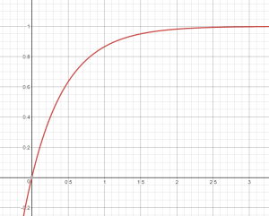
An SG integral is actually very cheap to compute…or at least it would be if we removed the exponential term. It turns out that the \( (1 - e^{-2\lambda}) \) term actually approaches 1 very quickly as the SG’s sharpness increases, which means we can potentially drop it with little error as long as we know that the sharpness is high enough. Here’s what a graph of \( (1 - e^{-2\lambda}) \) looks like for increasing sharpness:

This all lends itself naturally to HLSL implementations for accurate and approximate versions of an SG integral:

float3 SGIntegral(in SG sg)
{
    float expTerm = 1.0f - exp(-2.0f * sg.Sharpness);
    return 2 * Pi * (sg.Amplitude / sg.Sharpness) * expTerm;
}

float3 ApproximateSGIntegral(in SG sg)
{
    return 2 * Pi * (sg.Amplitude / sg.Sharpness);
}

Inner Product

If we were to use our SG integral formula to compute the integral of the product of two SG’s, we can compute what’s known as the inner product, or dot product of those SG’s. The operation is usually defined like this:

$$ \int_{\Omega} G_{1}(\mathbf{v}) G_{2}(\mathbf{v}) d\mathbf{v} = \frac{4 \pi a_{0} a_{1}}{e^{\lambda_{m}}} \frac{sinh(d_{m})}{d_{m}} $$

$$ d_{m} = || \lambda_{1}\mu_{1} + \lambda_{2}\mu_{2} || $$

However we can avoid numerical precision issues by using an alternate arrangement:

$$ \int_{\Omega} G_{1}(\mathbf{v}) G_{2}(\mathbf{v}) d\mathbf{v} = 2 \pi a_{0} a_{1}\frac{e^{d_{m} - \lambda_{m}} - e^{-d_{m} - \lambda_{m}}}{d_{m}} $$

…which looks like this in HLSL:

float3 SGInnerProduct(in SG x, in SG y)
{
    float dm = length(x.Sharpness * x.Axis + y.Sharpness * y.Axis);
    float3 expo = exp(dm - x.Sharpness - y.Sharpness) * x.Amplitude * y.Amplitude;
    float other = 1.0f - exp(-2.0f * dm);
    return (2.0f * Pi * expo * other) / dm;
}

Treshold

SG’s have what’s known as “compact-ε” support, which means that it’s possible to determine an angle θ such that all points within θ radians of the SG’s axis will have a value greater than ε. This property is potentially more useful if we flip it around so that we calculate a sharpness λ that results in a given θ for a particular value of ε:

$$ ae^{\lambda(cos\theta - 1)} = \epsilon $$ $$ \lambda = \frac{ln(\epsilon) - ln(a)}{cos\theta - 1} $$

float SGSharpnessFromThreshold(in float amplitude,
                               in float epsilon,
                               in float cosTheta)
{
    return (log(epsilon) - log(amplitude)) / (cosTheta - 1.0f);
}

Rotation

One last operation I’ll discuss is rotation. Rotating an SG is trivial: all you need to do is apply your rotation transform to the SG’s axis vector and you have a rotated SG! You can apply the transform using a matrix, a quaternion, or any other means you might have for rotating a vector. This is a welcome change from SH, which requires a very complex transform once you go above L1.

[1] Gaussian Function
[2] All-Frequency Rendering of Dynamic, Spatially-Varying Reflectance
[3] Error Function
[4] von-Mises Fisher Distribtion

Comments:

Mike R. - Nov 1, 2017

Just wanted say thanks for the awesome explanations, you make everything so clear and easy to understand.

Yes indeed, that was an error on my part. Thank you for pointing that out!

\( G_{1}(\mathbf{v})G_{2}(\mathbf{v}) = G(\mathbf{v};\frac{\mu_{m}}{||\mu_{m}||},a_{1}a_{2}e^{\lambda_{m}(||\mu_{m}|| - 1)}) \) is it lost the sharpness λm∥pm∥? and SG SGProduct(in SG x, in SG y) { float3 um = (x.Sharpness * x.Axis + y.Sharpness + y.Axis) / (x.Sharpness + y.Sharpness); is this should be: float3 um = (x.Sharpness * x.Axis + y.Sharpness * y.Axis) / (x.Sharpness + y.Sharpness);