SG Series Part 4: Specular Lighting From an SG Light Source

This is part 4 of a series on Spherical Gaussians and their applications for pre-computed lighting. You can find the other articles here:

Part 1 - A Brief (and Incomplete) History of Baked Lighting Representations
Part 2 - Spherical Gaussians 101
Part 3 - Diffuse Lighting From an SG Light Source
Part 4 - Specular Lighting From an SG Light Source
Part 5 - Approximating Radiance and Irradiance With SG’s
Part 6 - Step Into The Baking Lab

In the previous article, we explored a few ways to compute the contribution of an SG light source when using a diffuse BRDF. While this is already useful, it would be nice to be able work with more complex view-dependent BRDF’s so that we can also compute a specular contribution. In this article I’ll explain a possible approach for approximating the response of a microfacet specular BRDF when applied to an SG light, and also introduce the concept of Anisotropic Spherical Gaussians.

Microfacet Specular Recap

You probably recall from the past 5 years of physically based rendering presentations[1] that a standard microfacet BRDF takes the following structure:

$$ f(\mathbf{i}, \mathbf{o}) = \frac{F(\mathbf{o}, \mathbf{h})\,G(\mathbf{i}, \mathbf{o}, \mathbf{h})\,D(\mathbf{h})} {4\,(\mathbf{n} \cdot \mathbf{i})\,(\mathbf{n} \cdot \mathbf{o})} $$

Recall that D(h) is the distribution term, which tells us the percentage of active microfacets for a particular combination of view and light vectors. It’s also commonly known as the normal distribution function, or “NDF” for short. It’s generally parameterized on a roughness parameter, which essentially describes the “bumpiness” of the underlying microgeometry. Lower roughness values lead to sharp mirror-like reflections with a very narrow and intense specular lobe, while higher roughness values lead to more broad reflections with a wider specular lobe. Most modern games (including The Order: 1886) use the GGX (AKA Trowbridge-Reitz) distribution for this purpose.

Next we have G(i, o, h) which is referred to as the geometry term or the masking-shadow function. Eric Heitz’s paper on the masking-shadow function[2] has a fantastic explanation of how these terms work and why they’re important, so I would strongly recommend reading through it if you haven’t already. As Eric explains, the geometry term actually accounts for two different phenomena. The first is the local occlusion of reflections by other neighboring microfacets. Depending on the angle of the incoming lighting and the bumpiness of the microsurface, a certain amount of the lighting will be occluded by the surface itself, and this term attempts to model that. The other phenomenon handled by this term is visibility of the surface from the viewer. A surface that isn’t visible naturally can’t reflect light towards the viewer, and so the geometry term models this masking effect using the view direction and the roughness of the microsurface.

Finally we have F(o, h), which is the Fresnel term. This familiar term determines the amount of light that is reflected vs. the amount that is refracted or absorbed, which varies depending on the index of refraction for a particular interface as well as the angle of incidence. For a microfacet BRDF we compute the Fresnel term using the angle between the active microfacet direction (the half vector) and the light or view direction (it is equivalent to use either). This generally causes the reflected intensity  to increase when both the viewing direction and the light direction are grazing with respect to the surface normal. In real-time graphics Schlick’s approximation is typically used to represent the Fresnel term, since it’s a bit cheaper than evaluating the actual Fresnel equations. It is also common to parameterize the Fresnel term on the reflectance at zero incidence (referred to as “F0”) instead of directly working with an index of refraction.

Specular From an SG Light

Let’s now return to our example of a Spherical Gaussian light source. In the previous article we explored how to approximate the purely diffuse contribution from such a light source, but how do we handle the specular response? If we go down this road, we ideally want to do it in a way that uses a microfacet specular model so that we can remain consistent with our lighting from punctual light sources and IBL probes. If we start out by just plugging our BRDF and SG light into the rendering equation we get this monstrosity:

$$ L_{o}(\mathbf{o}, \mathbf{x}) = \int_{\Omega}  \frac{F(\mathbf{o}, \mathbf{h})\,G(\mathbf{i}, \mathbf{o}, \mathbf{h})\,D(\mathbf{h})G_{l}(\mathbf{i};\mathbf{\mu},\lambda,a)cos(\theta_{i})d\Omega} {4cos(\theta_{i})cos(\theta_{o})} $$

$$ L_{o}(\mathbf{o}, \mathbf{x}) = \int_{\Omega}  \frac{F(\mathbf{o}, \mathbf{h})\,G(\mathbf{i}, \mathbf{o}, \mathbf{h})\,D(\mathbf{h})ae^{\lambda(\mathbf{\mu} \cdot \mathbf{i} - 1)}d\Omega} {4cos(\theta_{o})} $$

Unlike diffuse we now have multiple terms inside the integral, many of which are view-dependent. This suggests that we will need to combine several aggressive optimizations in order to get anywhere close to our desired result.

The Distribution Term

Let’s start out by taking the distribution term on its own, since it’s arguably the most important part of the specular BRDF. The distribution determines the overall shape and intensity of the resulting specular highlight, and has a widely-varying frequency response over the domain of possible roughness values. If we look at the graph of the GGX distribution from the earlier section, the shape does resemble a Gaussian. Unfortunately it’s not an exact match: the GGX distribution has the characteristic narrow highlight and long  tails which we can’t match using a single SG. We could get a closer fit by summing multiple Gaussians, but for this article we’ll keep things simple by sticking with a single lobe. If we go back to Wang et al.’s paper[3] that we referenced earlier, we can see that they suggest a very simple fit of an SG to a Cook-Torrance distribution term:

$$ D(\mathbf{h})= e^{-(arccos(\mathbf{h} \cdot \mathbf{n})/m)^{2}} \approx G(\mathbf{h};\mathbf{n},\frac{2}{m^2},1) $$

If we look closely, we can see that they’re actually fitting for the Gaussian model mentioned in the original Cook-Torrance paper[4], which is similar to the one used in the Torrance-Sparrow model[5]. Note that this should not be confused the with Beckmann distribution that’s also mentioned in the Cook-Torrance paper, which is actually a 2D Gaussian in the slope domain (AKA parallel plane domain). However the shape isn’t even the biggest problem here, as the variant they’re using isn’t normalized. This means the peak of the Gaussian will always have a height of 1.0, rather than shrinking when the roughness increases and growing when the roughness decreases. Fortunately this is really easy to fix, since we have a simple analytical formula for computing the integral of an SG. Therefore if we set the amplitude to 1 over the integral, we end up with a normalized distribution:

$$ D_{SG}(\mathbf{h})= G(\mathbf{h};\mathbf{n},\frac{2}{m^2}, \frac{1}{\pi m^2}) $$

SG DistributionTermSG(in float3 direction, in float roughness)
{
    SG distribution;
    distribution.Axis = direction;
    float m2 = roughness * roughness;
    distribution.Sharpness = 2 / m2;
    distribution.Amplitude = 1.0f / (Pi * m2);

    return distribution;
}

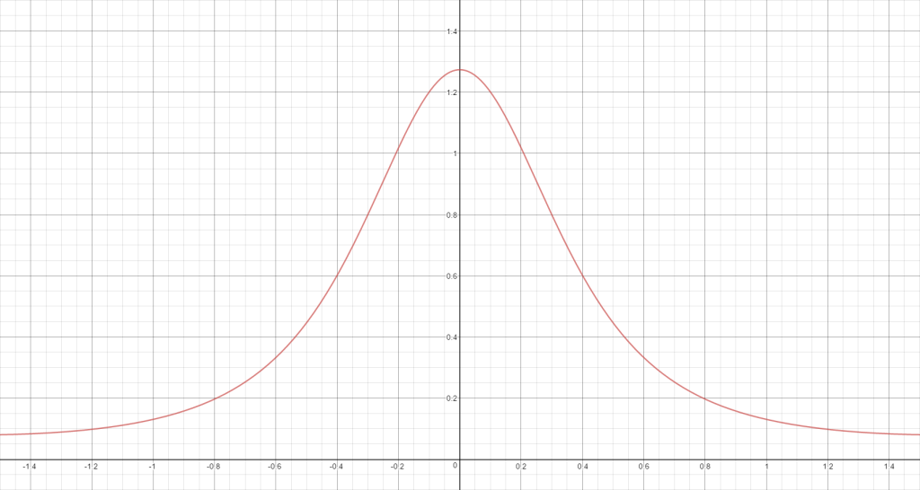
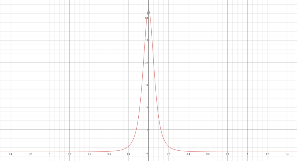
Let’s take a look at a graph of our distribution term, and see how far off it is from our target:

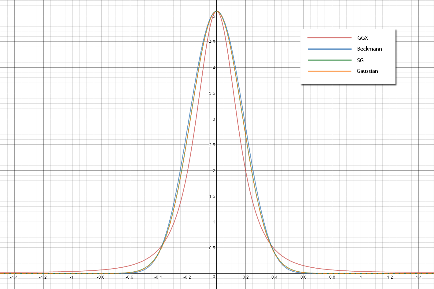
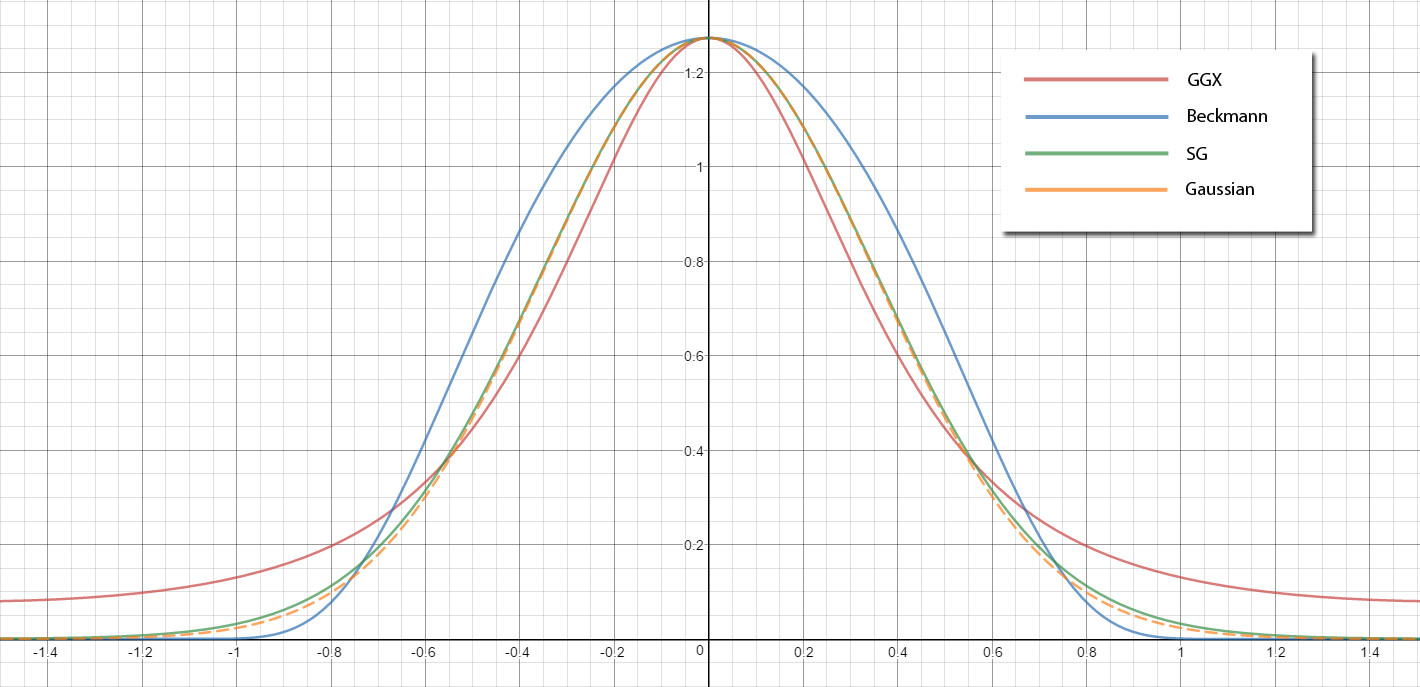
It should come as no surprise that our SG distribution is almost an exact match for a normalized version of a Gaussian distribution. When the roughness is lower it’s also a fairly close match for Beckmann, but for higher roughness the difference gets to be quite large. In both cases our distribution isn’t a perfect fit for GGX, but it’s a workable approximation.

Warping Between Domains

So we now have a normal distribution function in SG format, but unfortunately we’re not quite ready to use it as-is. The problem is that we’ve defined our distribution in the half-vector domain: the axis of the SG points in the direction of the surface normal, and we use the half-vector as our sampling direction. If we want to use an SG product to compute the result of multiplying our distribution with an SG light source, then we need to ensure that the distribution lobe is in the same domain as our light source. Another way to think about this is that center of our distribution shifts depending on viewing angle, since the half-vector also shifts as the camera moves.

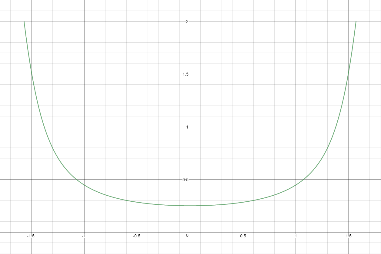
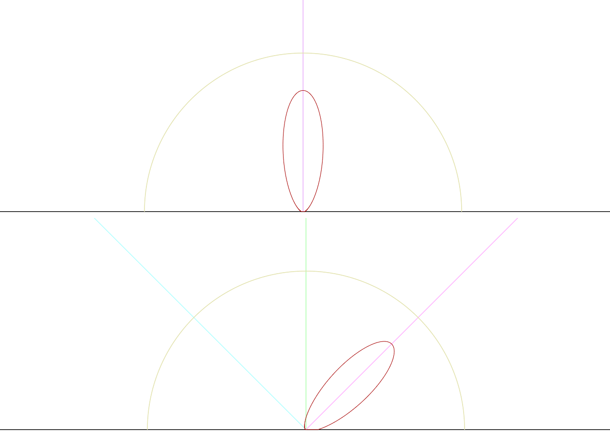
In order to make sure that our distribution lobe is in the correct domain, we need “warp” our distribution so that it lines up with the current BRDF slice for our viewing direction. If you’re wondering what a BRDF slice is, it basically tells you “if I pick a particular view direction. what is the value of my  BRDF for a given light direction?”. So if you had a mirror BRDF, the slice would just be a single ray pointing in the direction of the view ray reflected off the surface normal. For microfacet specular BRDF’s, you get a lobe that’s roughly centered around the reflected view direction. Here’s what a polar graph of a GGX BRDF slice looks like if we only consider the distribution term:

Wang et al. proposed a simple spherical warp operator that would orient the distribution lobe about the reflected view direction, while also modifying the sharpness to take into account the differential area at the original center of the lobe:

$$ \mu_{w}=2(\mathbf{o} \cdot \mu_{d})\mu_{d} - \mathbf{o} $$

$$ \lambda_{w}=\frac{\lambda_{d}}{4|\mu_{d} \cdot \mathbf{o}|} $$

$$ a_{w} = a_{d} $$

SG WarpDistributionSG(in SG ndf, in float3 view)
{
    SG warp;

    warp.Axis = reflect(-view, ndf.Axis);
    warp.Amplitude = ndf.Amplitude;
    warp.Sharpness = ndf.Sharpness;
    warp.Sharpness /= (4.0f * max(dot(ndf.Axis, view), 0.0001f));

    return warp;
}

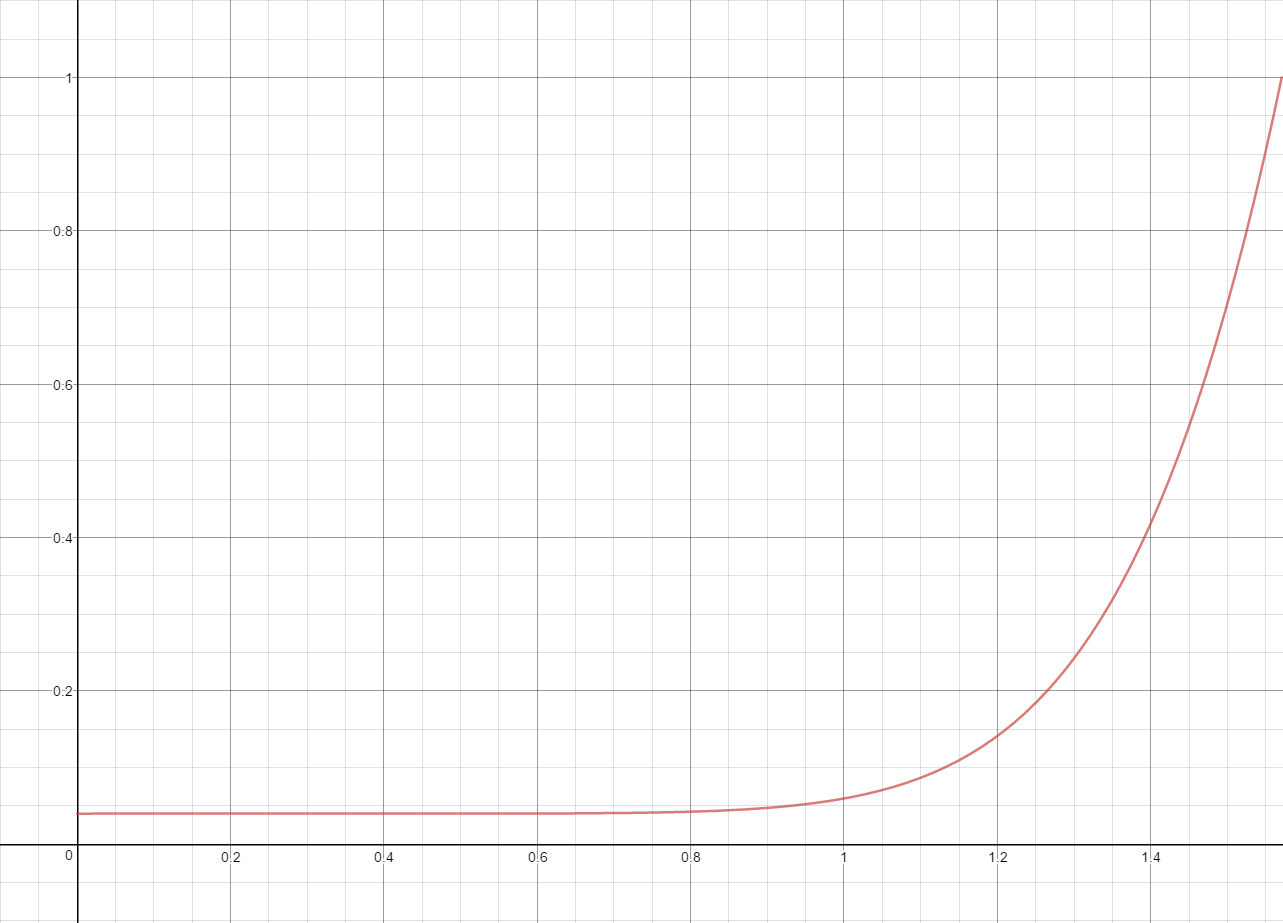
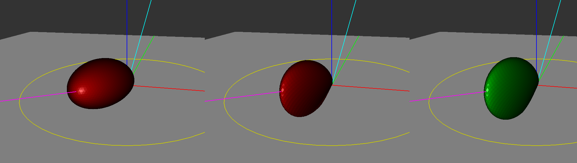
Let’s now look at the result of that warp, and compare it to what the actual GGX distribution looks like:

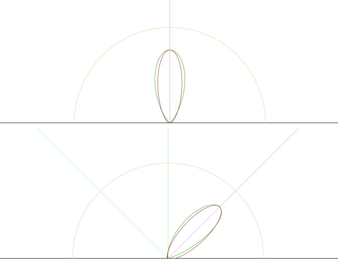
A quick look at the graph shows us that the shape is a bit off, but our warped lobe is ending up in approximately in the right spot. We’ll revisit the lobe shape later, but for now let’s try combining our distribution with the rest of our BRDF.

Approximating The Remaining Terms

In the previous section we figured out how to obtain an SG approximation of our distribution term, and also warp it so that it’s in the correct domain for multiplication with our SG light source. Using our SG product operator would allow to us to represent the result of multiplying the distribution with the light source as another SG, which we could then multiply with other terms using SG operators…or at least we could if we were to represent the remaining terms as SG’s. Unfortunately this turns out to be a problem: the geometry and Fresnel terms are nothing at all like a Gaussian, which rules out approximating them as an SG. Wang et al. sidestep this issue by making the somewhat-weak assumption that the values of these terms will be constant across the entire BRDF lobe, which allows them to pull the terms out of the integral and evaluate them only for the axis direction of the BRDF lobe. This allows the resulting BRDF to still capture some of the glancing angle effects, with similar performance cost to evaluating those terms for a punctual light source. The downside is that the error of these terms will increase as the BRDF lobe becomes wider (increasing roughness), since the value of the geometry and Fresnel terms will vary more the further they are from the lobe center. Putting it all together gives the following specular BRDF:

$$ f_{sg}(\mathbf{i}, \mathbf{o}) = \frac{F(\mathbf{o}, \mathbf{h_{w}})\,G(\mathbf{\mu_{w}}, \mathbf{o}, \mathbf{h_{w}})\, \frac{1}{\pi m^2}e^{\lambda_{w}(\mathbf{\mu_{w}} \cdot \mathbf{i} - 1)}} {4\,(\mathbf{n} \cdot \mathbf{\mu_{w}})\,(\mathbf{n} \cdot \mathbf{o})} $$

$$ \mathbf{h_{w}} = \frac{\mathbf{o} + \mathbf{\mu_{w}}}{||\mathbf{o} + \mathbf{\mu_{w}}||} $$

The last thing we need to account for is the cosine term that needs to be multiplied with the BRDF inside of the hemispherical integral. Wang et al. suggest using an SG product to compute an SG representing the result of multiplying the distribution term SG and their SG approximation of a clamped cosine lobe, which can then be multiplied with the lighting lobe using an SG inner product. In order to avoid another expensive SG operation, we will instead use the same approach that we used for geometry and Fresnel terms and evaluate the cosine term using the BRDF lobe axis direction. Implementing it in shader code gives us the following:

float GGX_V1(in float m2, in float nDotX)
{
    return 1.0f / (nDotX + sqrt(m2 + (1 - m2) * nDotX * nDotX));
}

float3 SpecularTermSGWarp(in SG light, in float3 normal,
                          in float roughness, in float3 view,
                          in float3 specAlbedo)
{
    // Create an SG that approximates the NDF.
    SG ndf = DistributionTermSG(normal, roughness);

    // Warp the distribution so that our lobe is in the same
    // domain as the lighting lobe
    SG warpedNDF = WarpDistributionSG(ndf, view);

    // Convolve the NDF with the SG light
    float3 output = SGInnerProduct(warpedNDF, light);

    // Parameters needed for the visibility
    float3 warpDir = warpedNDF.Axis;
    float m2 = roughness * roughness;
    float nDotL = saturate(dot(normal, warpDir));
    float nDotV = saturate(dot(normal, view));
    float3 h = normalize(warpedNDF.Axis + view);

    // Visibility term evaluated at the center of
    // our warped BRDF lobe
    output *= GGX_V1(m2, nDotL) * GGX_V1(m2, nDotV);

    // Fresnel evaluated at the center of our warped BRDF lobe
    float powTerm = pow((1.0f - saturate(dot(warpDir, h))), 5);
    output *= specAlbedo + (1.0f - specAlbedo) * powTerm;

    // Cosine term evaluated at the center of the BRDF lobe
    output *= nDotL;

    return max(output, 0.0f);
}

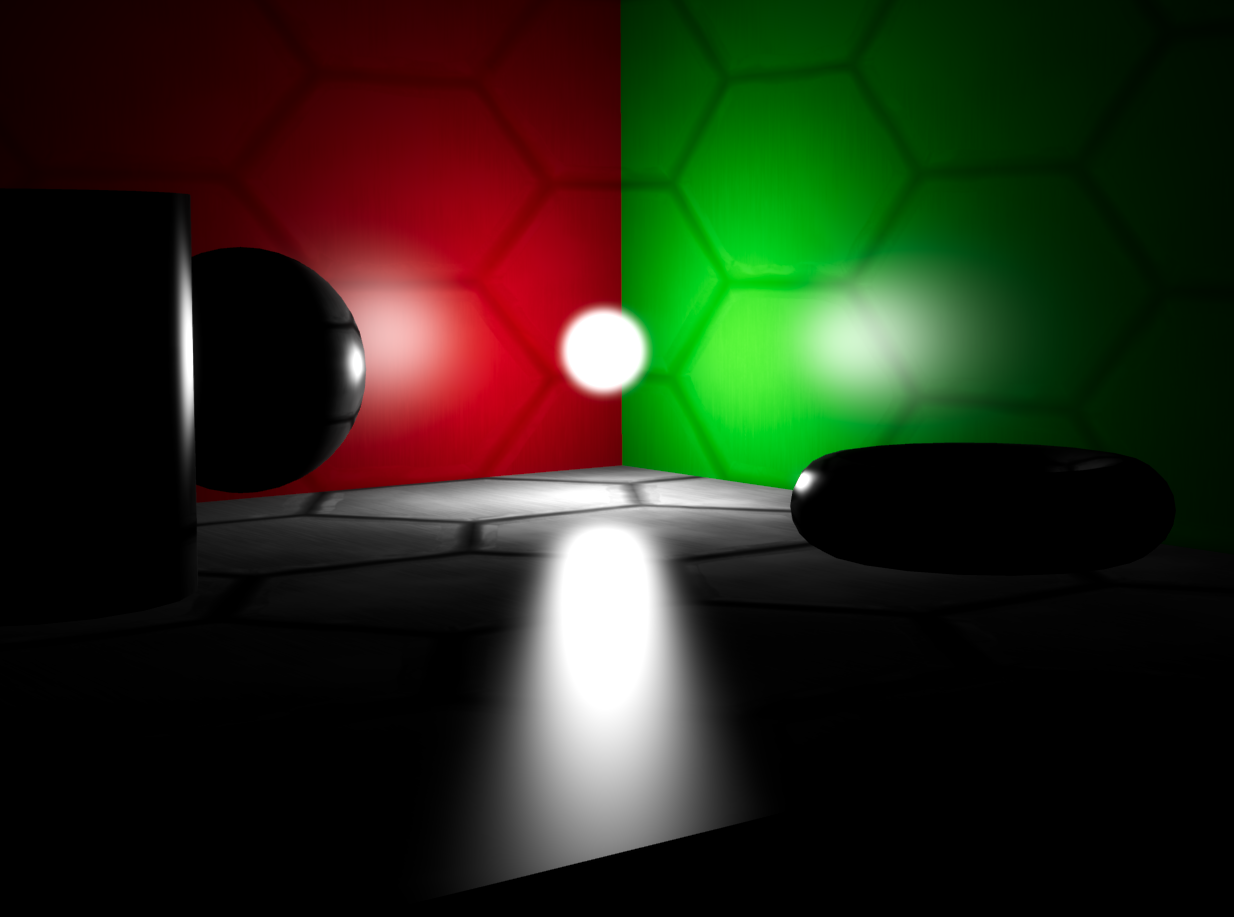
Let’s now (finally) take a look at what our specular approximation looks like for a scene being lit by an SG light source:

Going Anisotropic

So if we look at the specular highlights in the above image, you may notice that while the highlights on the red and green walls look pretty good, the highlight on floor seems a bit off. The highlight is rather wide and rounded, and our intuition tells that a highlight viewed at a grazing angle should appear vertically stretched across the floor. To determine why the look is so off, we need to revisit our warp of the distribution term. Previously when we looked at the polar graph of the distribution I noted that the shape of the resulting lobe was a bit off, even though it was oriented in approximately the right direction to line up with the BRDF slice. To get a better idea of what’s going on, let’s now take a look at a 3D graph of the GGX distribution term:

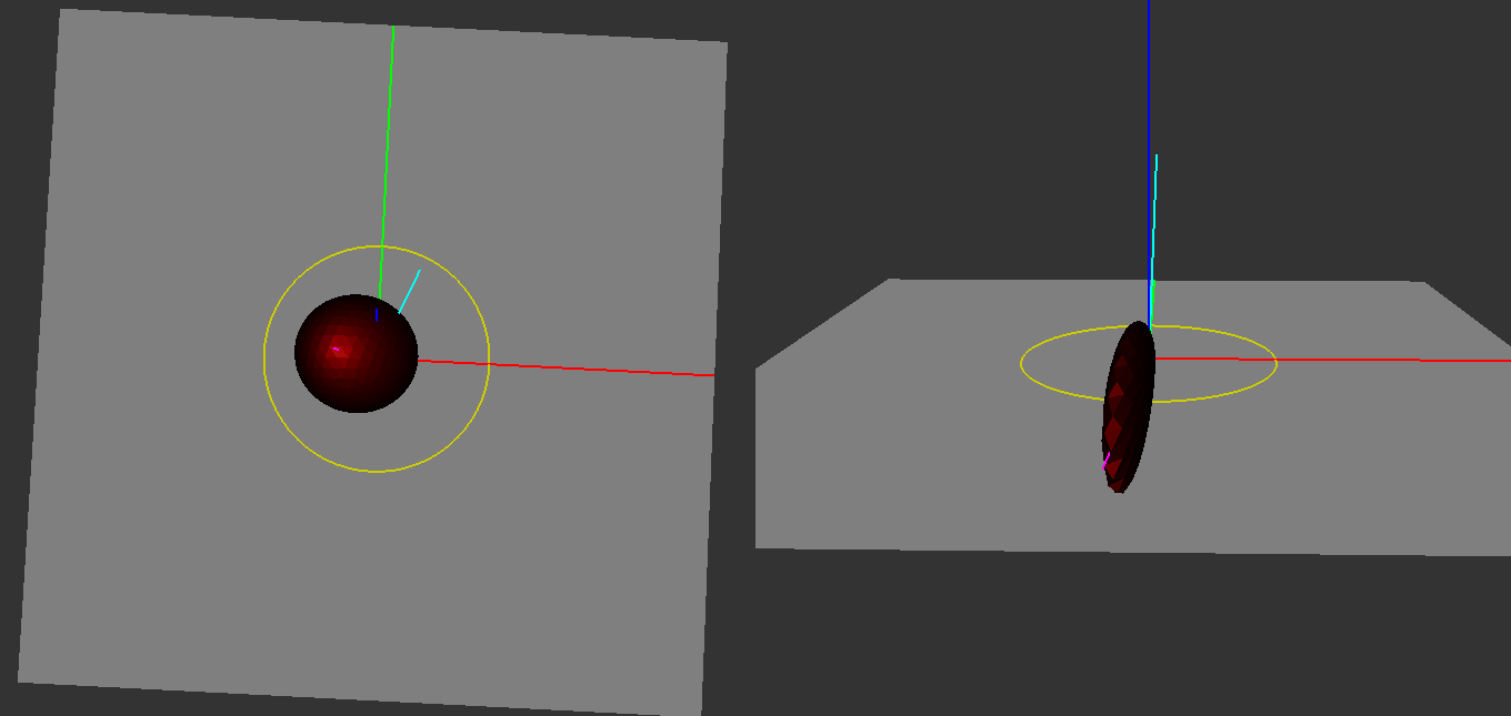
Looking at the left image where the angle between the view direction and  the surface normal are very low, the distribution is radially symmetrical just like an SG lobe. However as the viewing angle increases the lobe begins to stretch, looking more and more like the non-symmetrical lobe that we see in the right image. The stretching of the lobe is what causes the stretched highlights that occur when applying the BRDF, and our warped SG is unable to properly represent it since it must remain radially symmetric about its axis.

Luckily for us, there is a better way. In 2013 Xu et al.released a paper titled Anisotropic Spherical Gaussians[6], where they explain how they extended SG’s to support anisotropic lobe width/sharpness. They’re defined like this:

$$ G(\mathbf{v};[\mu_x, \mu_y, \mu_z],[\lambda_x, \lambda_y],a) = a \cdot S(\mathbf{v},\mu_z) e^{-\lambda_x(\mathbf{v} \cdot \mu_x) - \lambda_y(\mathbf{v} \cdot \mu_y)} $$

Instead of having a single axis direction, an ASG now has \(  \mu_x &s=1 $, \(  \mu_y \), and \(  \mu_z \), which are three orthogonal vectors forming a complete basis. It’s very similar to a tangent frame, where the normal, tangent, and bitangent together make up an orthonormal basis. With an ASG you also now have two separate sharpness parameters, \(  \lambda_x \) and \( \lambda_y \), which control the sharpness with respect to \(  \mu_x \) and \(  \mu_y \). So for example setting \(  \lambda_x \) to 16 and \( \lambda_y \) to 64 will result in stretched Gaussian lobe that’s skinnier along the \( \lambda_y \) direction, and with its center located at \(  \mu_z \). Visualizing such an ASG on the surface of a sphere gives you this:

Like SG’s, the equations lend themselves to simple HLSL implementations:

struct ASG
{
    float3 Amplitude;
    float3 BasisZ;
    float3 BasisX;
    float3 BasisY;
    float SharpnessX;
    float SharpnessY;
};

float3 EvaluateASG(in ASG asg, in float3 dir)
{
    float sTerm = saturate(dot(asg.BasisZ, dir));
    float lambdaTerm = asg.SharpnessX * dot(dir, asg.BasisX) * dot(dir, asg.BasisX);
    float muTerm = asg.SharpnessY * dot(dir, asg.BasisY) * dot(dir, asg.BasisY);
    return asg.Amplitude * sTerm * exp(-lambdaTerm - muTerm);
}

The ASG paper provides us with formulas for two operations that we can use to improve the quality of our specular approximation for SG light sources. The first is a new warping operator that can take an NDF represented as an isotropic SG, and stretch it along the view direction to produce an ASG that better represents the actual BRDF. The other helpful forumula it provides is for convolving an ASG with an SG, which we can use to convolve a anisotropically warped NDF lobe with an SG lighting lobe. Let’s take a look at how their improved warp looks when graphing the NDF for a large viewing angle:

The anisotropic distribution looks much closer to the actual GGX NDF, since it now has the vertical stretching that we were missing. Let’s now implement their formulas in HLSL so we can try the new warp in our test scene:

float3 ConvolveASG_SG(in ASG asg, in SG sg) {
    // The ASG paper specifes an isotropic SG as
    // exp(2 * nu * (dot(v, axis) - 1)),
    // so we must divide our SG sharpness by 2 in order
    // to get the nup parameter expected by the ASG formula
    float nu = sg.Sharpness * 0.5f;

    ASG convolveASG;
    convolveASG.BasisX = asg.BasisX;
    convolveASG.BasisY = asg.BasisY;
    convolveASG.BasisZ = asg.BasisZ;

    convolveASG.SharpnessX = (nu * asg.SharpnessX) / (nu + asg.SharpnessX);
    convolveASG.SharpnessY = (nu * asg.SharpnessY) / (nu + asg.SharpnessY);

    convolveASG.Amplitude = Pi / sqrt((nu + asg.SharpnessX) *
    (nu + asg.SharpnessY));

    float3 asgResult = EvaluateASG(convolveASG, sg.Axis);
    return asgResult * sg.Amplitude * asg.Amplitude;
}

ASG WarpDistributionASG(in SG ndf, in float3 view)
{
    ASG warp;

    // Generate any orthonormal basis with Z pointing in the
    // direction of the reflected view vector
    warp.BasisZ = reflect(-view, ndf.Axis);
    warp.BasisX = normalize(cross(ndf.Axis, warp.BasisZ));
    warp.BasisY = normalize(cross(warp.BasisZ, warp.BasisX));

    float dotDirO = max(dot(view, ndf.Axis), 0.0001f);

    // Second derivative of the sharpness with respect to how
    // far we are from basis Axis direction
    warp.SharpnessX = ndf.Sharpness / (8.0f * dotDirO * dotDirO);
    warp.SharpnessY = ndf.Sharpness / 8.0f;

    warp.Amplitude = ndf.Amplitude;

    return warp;
}

float3 SpecularTermASGWarp(in SG light, in float3 normal,
                           in float roughness, in float3 view,
                           in float3 specAlbedo)
{
    // Create an SG that approximates the NDF
    SG ndf = DistributionTermSG(normal, roughness);

    // Apply a warpring operation that will bring the SG from
    // the half-angle domain the the the lighting domain.
    ASG warpedNDF = WarpDistributionASG(ndf, view);

    // Convolve the NDF with the light
    float3 output = ConvolveASG_SG(warpedNDF, light);

    // Parameters needed for evaluating the visibility term
    float3 warpDir = warpedNDF.BasisZ;
    float m2 = roughness * roughness;
    float nDotL = saturate(dot(normal, warpDir));
    float nDotV = saturate(dot(normal, view));
    float3 h = normalize(warpDir + view);

    // Visibility term
    output *= GGX_V1(m2, nDotL) * GGX_V1(m2, nDotV);

    // Fresnel
    float powTerm = pow((1.0f - saturate(dot(warpDir, h))), 5);
    output *= specAlbedo + (1.0f - specAlbedo) * powTerm;

    // Cosine term
    output *= nDotL;

    return max(output, 0.0f);
}

If we swap out our old specular approximation for one that uses an anisotropic warp, our test scene now looks much better!

Visually Comparing the BRDF

Many of the images that I used for visually comparing the SG BRDF approximations were generated using Disney’s BRDF Explorer. When we were doing our initial research into SG’s and figuring out how to implement them, BRDF Explorer was extremely valuable both for understanding the concepts and for experimenting with different variations. If you’d like to this yourself, there’s a very easy way to do that courtesy of Nick Brancaccio. Nick was kind of enough to create his own awesome WebGL version of BRDF Explorer, and it comes pre-loaded with options for comparing an approximate SG specular BRDF with the GGX BRDF. I would recommend checking it out if you’d like to play around with the BRDF’s and make some pretty 3D graphs!

Update 07/04/2023: it appears that the URL for the WebGL BRDF explorer no longer works, and is likely gone forever

References

[1] Background: Physics and Math of Shading (SIGGRAPH 2013 Course: Physically Based Shading in Theory and Practice)
[2] Understanding the Masking-Shadowing Function in Microfacet-Based BRDFs
[3] All-Frequency Rendering of Dynamic, Spatially-Varying Reflectance
[4] A Reflectance Model for Computer Graphics
[5] Theory for Off-Specular Reflection From Roughened Surfaces
[6] Anisotropic Spherical Gaussians
[7] BRDF Explorer
[8] WebGL BRDF Explorer (defunct)

Comments:

MJP - Oct 1, 2016

Thank you Evgenii! I added the missing link. I’m also glad that you like the graphs, it took a while to generate all of them. :)

The first paragraph is missing a link. :-) Great series! I especially like the included graphs.

Hi MJP, I’ve noticed that we could fit more gaussians to an arbitrary function. For example I’ve managed to match the Beckmann distribution with 3 gaussians for the roughness value of 1 https://www.desmos.com/calculator/o1lces1o1l My aim is to fit between 2-5 gaussians to common BRDFs and sample from environment maps pre-convolved with SG, then that way I can get a much better approximation to Importance Sampled references than the current IBL methods.