SG Series Part 3: Diffuse Lighting From an SG Light Source

This is part 3 of a series on Spherical Gaussians and their applications for pre-computed lighting. You can find the other articles here:

Part 1 - A Brief (and Incomplete) History of Baked Lighting Representations
Part 2 - Spherical Gaussians 101
Part 3 - Diffuse Lighting From an SG Light Source
Part 4 - Specular Lighting From an SG Light Source
Part 5 - Approximating Radiance and Irradiance With SG’s
Part 6 - Step Into The Baking Lab

A Big Gaussian In The Sky

In the previous post we covered a few of the universal properties of SG’s. Now that we have a few tools on our utility belt, let’s discuss an example of how we can actually use those properties to our advantage in a rendering scenario. Let’s say we have a surface point x being lit by a light source L, with the light source being represented by an SG named GL. Recall from the previous article that the equation for computing the outgoing radiance towards the eye for a surface with a Lambertian diffuse BRDF looks like the following:

$$ L_{o}(\mathbf{o}, \mathbf{x}) = \frac{C_{diffuse}}{\pi} \int_{\Omega} L_{i}(\mathbf{i}, \mathbf{x})cos(\theta_{i})d\Omega $$

For punctual light sources that are essentially a scaled delta function, computing this is as easy as N dot L. But we’re in trouble if we have an area light source, since we typically don’t have a closed form solution to the integral. But let’s suppose that we have some strange Gaussian light source, whose angular falloff can be exactly represented by an SG (normally area light sources are considered  to have uniform emission over their surface, but let’s imagine we have case where the emission is non-uniform). If we can treat the light as an SG, then we can start to consider some of the handy Gaussian tools that we laid out earlier. In particular the inner product starts to seem really useful: it gives us the result of integrating the product of two SG’s, which is basically what we’re trying to accomplish in our diffuse lighting equation. The big catch is that we’re not integrating the product of two SG’s, we’re instead integrating the product of an SG with a clamped cosine lobe. Obviously a Gaussian lobe has a different shape compared to a clamped cosine lobe, but perhaps if we squint our eyes from a distance you could substitute one for another. This approach was taken by Wang et al.[1], who suggested fitting a cosine lobe to a single SG with λ=2.133 and a=1.17. If we follow in their footsteps, the diffuse calculation is straightforward:

SG CosineLobeSG(in float3 direction)
{
    SG cosineLobe;
    cosineLobe.Axis = direction;
    cosineLobe.Sharpness = 2.133f;
    cosineLobe.Amplitude = 1.17f;

    return cosineLobe;
}

float3 SGIrradianceInnerProduct(in SG lightingLobe, in float3 normal)
{
    SG cosineLobe = CosineLobeSG(normal);
    return max(SGInnerProduct(lightingLobe, cosineLobe), 0.0f);
}

float3 SGDiffuseInnerProduct(in SG lightingLobe, in float3 normal, in float3 albedo)
{
    float3 brdf = albedo / Pi;
    return SGIrradianceInnerProduct(lightingLobe, normal) * brdf;
}

Error Analysis

Not too bad, eh? Of course it’s worth taking a closer look at our cosine lobe approximation, since that’s definitely going to introduce some error. Perhaps the best way to do this is to look at the graphs of a real cosine lobe and our SG approximation side-by-side:

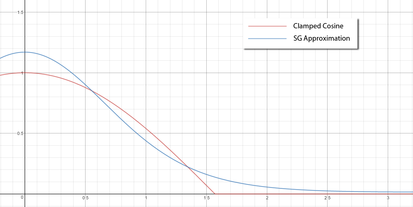
Just from looking at the graph it’s fairly obvious that an SG isn’t necessarily a great fit for a cosine lobe. First of all, the amplitude actually goes above 1, which might seem a bit weird at first glance. However it’s necessary to ensure that the area under the curve remains somewhat consistent with the cosine lobe, since there would otherwise be a loss of energy. The other weirdness stems from the fact that an SG never actually hits 0 anywhere on the sphere, hence the long “tail” on the graph of the SG. This essentially means that if the SG were integrated against a punctual light source, the lighting would “wrap” around the sphere past the point where N dot L is equal to 0. The situation actually isn’t all that different from an SH representation of a cosine lobe, which also extends past π/2:

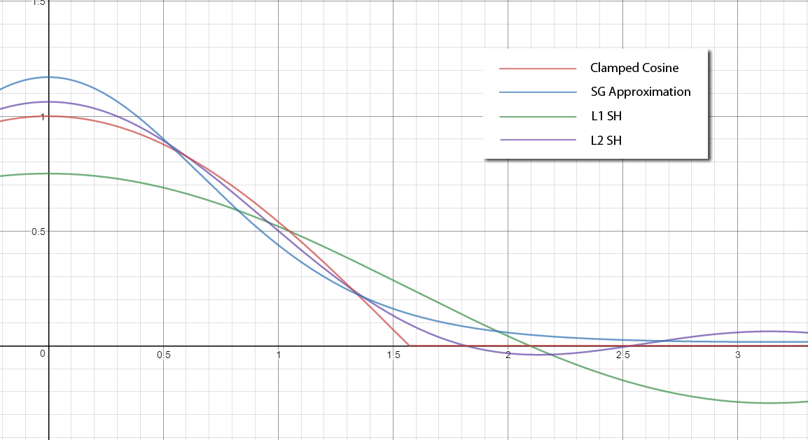
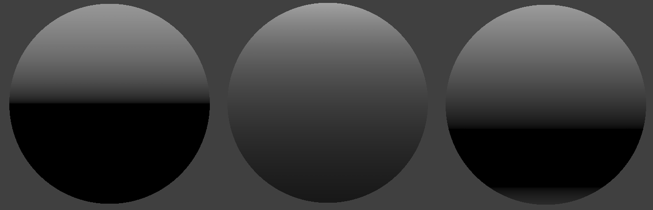
In the SH case the approximation actually goes negative, which is arguably worse than the long tail of the SG approximation. The L1 approximation is particularly bad in this regard. If at this point you’re trying to imagine what these approximations look like on a sphere, let me save you the trouble by providing an image:

Now that we’ve finished analyzing the approximation of a cosine lobe, we need to take a look at the actual results of computing diffuse lighting from an SG light source. Let’s start off by graphing the results of computing irradiance using an SG inner product, and compare it against what we get by using brute-force numerical integration to compute the result of multiplying the SG with an actual clamped cosine (not the approximate SG cosine lobe that we use for the inner product):

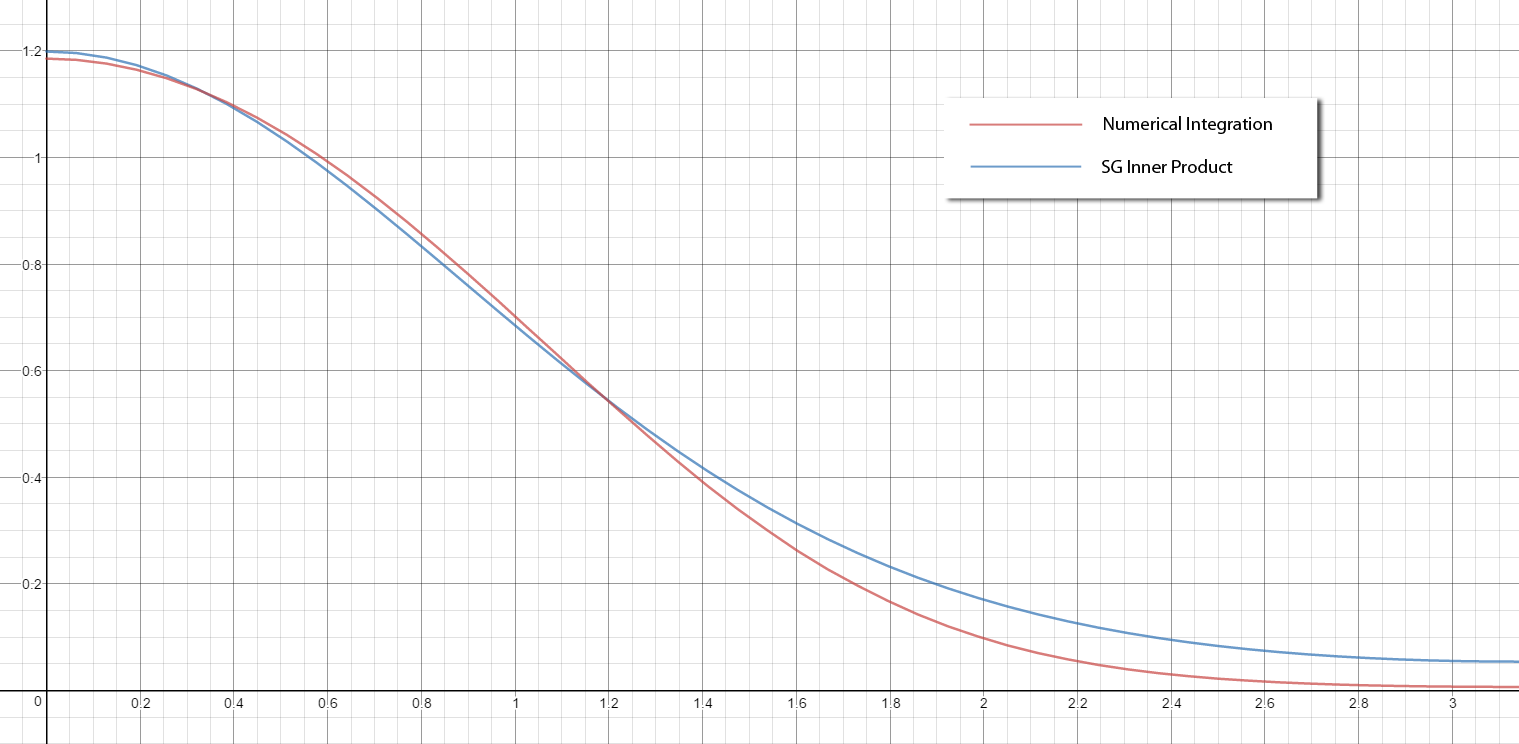
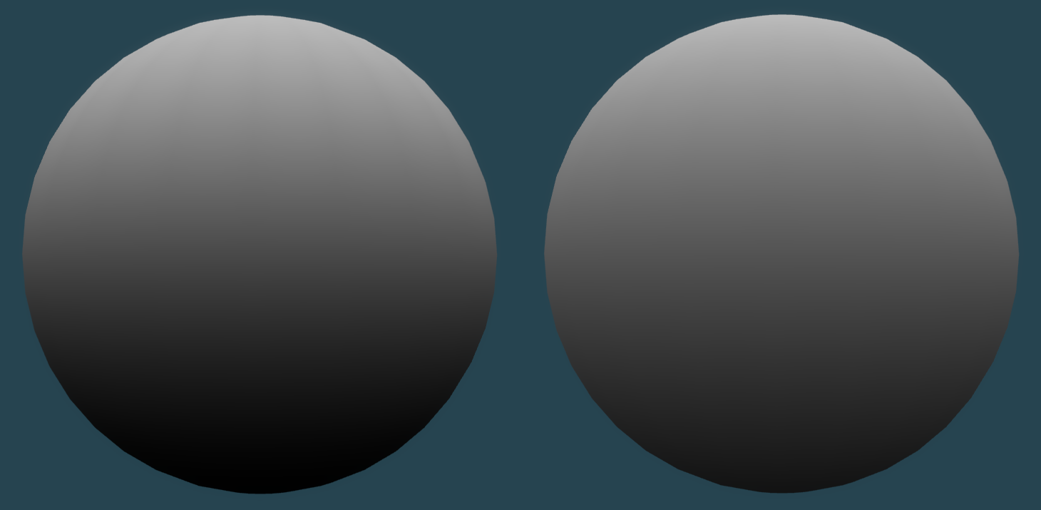
As you might expect, the inner product approximation has some error when compared with the “ground truth” provided by numerical integration. It’s worth pointing out that this error is purely a consequence of approximating the clamped cosine lobe as an SG: the inner product provides the exact result of the integral, and thus shouldn’t introduce any error on its own. Despite this error, the resulting irradiance isn’t hugely far off from our ground truth. The biggest difference is for the angles facing away from the light, where the SG inner product version has a stronger tail. Visualizing the resulting diffuse on a sphere gives us the following:

A Cheaper Approximation

As an alternative to representing the cosine lobe with an SG and computing the inner product, we can consider a cheaper approximation. One advantage of working with SG’s is that each lobe is always symmetrical about its axis, which is also where its value is the highest. We also discussed earlier how we can compute the integral of an SG over the sphere, which gives us its total energy. This suggests that if we want to be frugal with our shader cycles, we can pull terms out of the integral over the sphere/hemisphere and only evaluate them for the SG axis direction. This obviously introduces error, but that error may be acceptable if the term we pull out is relatively “smooth”. If we apply this approximation to computing irradiance and diffuse lighting, we get this:

$$ L_{o}(\mathbf{o}, \mathbf{x}) = \frac{C_{diffuse}}{\pi} \int_{\Omega} G_{L}(\mathbf{i};\mathbf{\mu},\lambda,a)cos(\theta_{i})d\Omega $$

$$ L_{o}(\mathbf{o}, \mathbf{x}) \approx cos(\theta_{\mu}) \frac{C_{diffuse}}{\pi} \int_{\Omega} G_{L}(\mathbf{i};\mathbf{\mu},\lambda,a)d\Omega $$

Translating to HLSL, we get the following functions:

float3 SGIrradiancePunctual(in SG lightingLobe, in float3 normal)
{
    float cosineTerm = saturate(dot(lightingLobe.Axis, normal));
    return cosineTerm * 2.0f * Pi * (lightingLobe.Amplitude) /
    lightingLobe.Sharpness;
}

float3 SGDiffusePunctual(in SG lightingLobe, in float3 normal, in float3 albedo)
{
    float3 brdf = albedo / Pi;
    return SGIrradiancePunctual(lightingLobe, normal) * brdf;
}

If we overlay the graph of our super-cheap irradiance approximation on the graph we were looking at earlier, we get this:

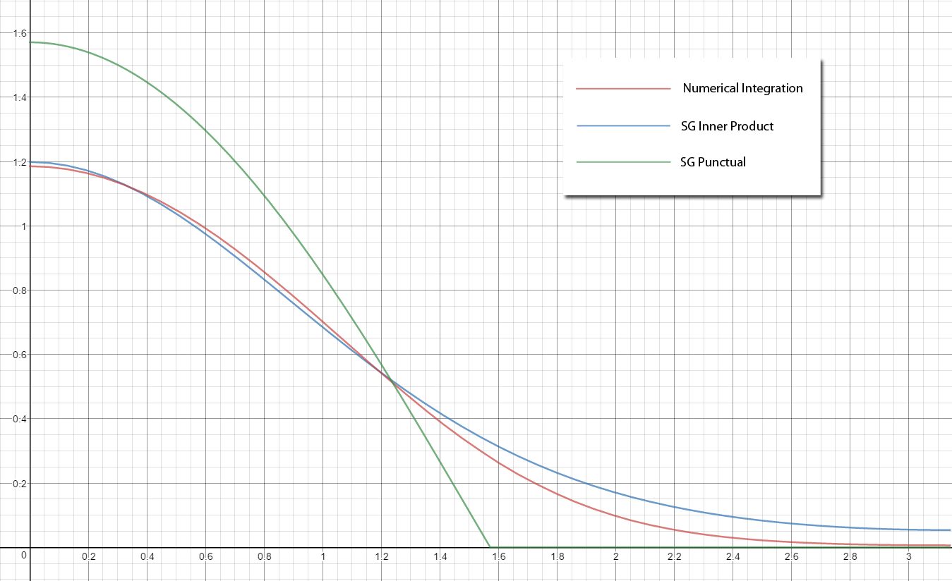
The result shouldn’t be a surprise: it’s just a scaled version of the standard clamped cosine.It’s pretty obvious just by looking that this particular optimization will introduce quite a bit of error, particularly where theta is greater than π/2. But it is cheap, since we’ve effectively turned an SG into a point light. This is makes it a useful tool for cases where we may want to approximate the convolution of an SG light source with a BRDF or some other function that isn’t easily represented as an SG.

A More Accurate Approximation

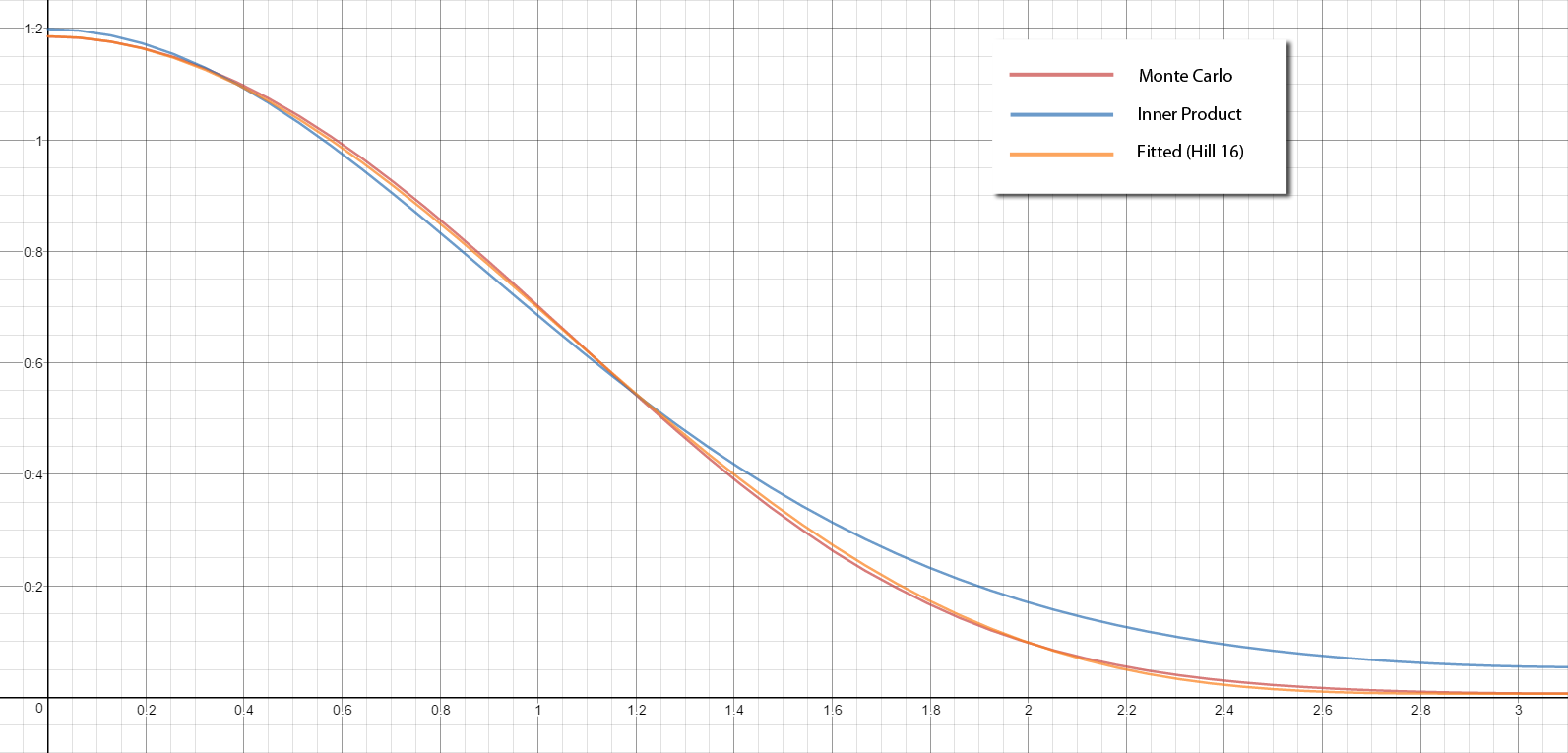
So it’s nice to have a cheap option, but what if we want more accuracy than our inner product approximation? Fortunately for us, Stephen Hill was able to formulate another alternative approximation that directly fits a curve to the integral of a cosine lobe with an SG. His implementation is actually formulated for a normalized SG (where the integral about the sphere is equal to 1.0), but we can easily account for this by computing the integral and scaling the result by that value:

float3 SGIrradianceFitted(in SG lightingLobe, in float3 normal)
{
    const float muDotN = dot(lightingLobe.Axis, normal);
    const float lambda = lightingLobe.Sharpness;

    const float c0 = 0.36f;
    const float c1 = 1.0f / (4.0f * c0);

    float eml = exp(-lambda);
    float em2l = eml * eml;
    float rl = rcp(lambda);

    float scale = 1.0f + 2.0f * em2l - rl;
    float bias = (eml - em2l) * rl - em2l;

    float x = sqrt(1.0f - scale);
    float x0 = c0 * muDotN;
    float x1 = c1 * x;

    float n = x0 + x1;

    float y = saturate(muDotN);
    if(abs(x0) <= x1)
    y = n * n / x;

    float result = scale * y + bias;

    return result * ApproximateSGIntegral(lightingLobe);
}

The result is very close to the ground truth, which is very cool considering that it might actually be cheaper than our inner product approximation!

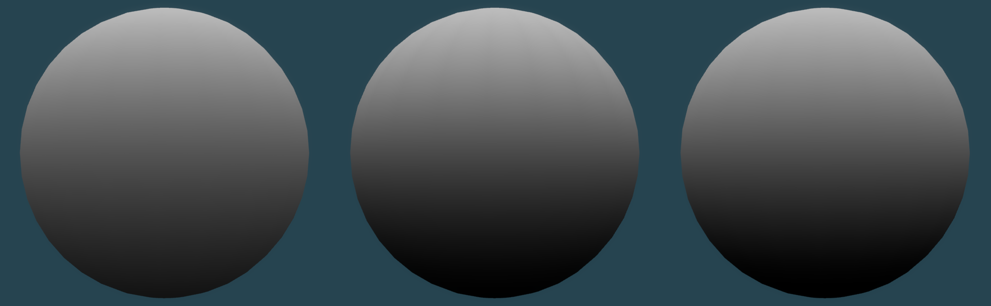
If we once again visualize the result on the sphere and compare with our previous results, we get the following:

References

[1] All-Frequency Rendering of Dynamic, Spatially-Varying Reflectance

Comments:

Stefan Dyulgerov - Oct 1, 2017

Hey, great article and nicely explained. 1. Can you update the links to the wang paper, since john snyders web site is reworked 2. Can you point a link to the SGIrradianceFitted, since the selfshadow is also updated.

Hi Stefan, I updated the link to Wang et al.’s paper. Thank you for pointing that out! As for Stephen Hill’s fitted SG irradiance approximation, the link that I currently have in there just points to his home page, which is still the same. He hasn’t formally published his approximation anywhere, so I don’t have anything else to link to at the moment.

In the second code listening “SGDiffusePunctual” should call “SGIrradiancePunctual” not “ApproximateSGIrradiance”, right? :) Great article series! :)

Yes, that’s right. I had renamed that function in the original source code, and neglected to properly update the code embedded in the article. Thank you for pointing that out, and also for the kind words. :)

Hi Matt, I definitely see how that could be confusing, now that you’ve pointed it out. I changed the text a bit to explicitly state that the graph represents the numerical integration of the SG light multiplied with the clamped cosine, so hopefully it will be a bit more clear for other readers. Either way I really appreciate the feedback! I should also thank you for writing such an amazing book, and making the complete source code available for reference! Without it I’m not sure if I would have gotten my own little path tracer working in the demo. :)

(Great series!) I was initially confused by your graph comparing numerical integration with the SG inner product–“shouldn’t numerical integration give the same result, since the inner product is exact and in closed form?” I asked myself; it wasn’t clear that you were comparing the integration of two different functions. I eventually figured out that you were numerically integrating the SG light model with the actual clamped cosine and comparing that to the inner product of the SG light and the SG clamped cosine (I think!); it might be nice to clarify the text/caption about that part of it. (On to part 4!)