SG Series Part 5: Approximating Radiance and Irradiance With SG's
This is part 5 of a series on Spherical Gaussians and their applications for pre-computed lighting. You can find the other articles here:
Part 1 - A Brief (and Incomplete) History of Baked Lighting Representations
Part 2 - Spherical Gaussians 101
Part 3 - Diffuse Lighting From an SG Light Source
Part 4 - Specular Lighting From an SG Light Source
Part 5 - Approximating Radiance and Irradiance With SG’s
Part 6 - Step Into The Baking Lab
In the two previous articles I showed workable approaches for approximating the diffuse and specular result from a Spherical Gaussian light source. On its own these techniques might seem a bit silly, since it’s not immediately obvious why the heck it would be useful to light a scene with an SG light source. But then you might remember that these articles started off by discussing methods for storing pre-computed radiance or irradiance in lightmaps or probe grids, which is a subject we’ll finally return to.
Finding The Perfect Fit
A common process in mathematics (particularly statistics) is to take a set of data points and attempt to figure out some sort of analytical curve that can represent the data. This process is known as curve fitting[1], since the goal is to find a curve that is a good fit for the data points. There’s various reasons to do this (such as regression analysis[2]), but I find it can helpful to think of it as a form of lossy compression: a few hundred data points might require kilobytes of data, but if you can approximate that data with a curve the coefficients might only need a few bytes of storage. Here’s a simple example from Wikipedia:

Fitting various polynomials to data generated by a sine wave. Red is first degree, green is second degree, orange is third degree, blue is forth degree. By Krishnavedala (Own work) [CC0], via Wikimedia Commons
In the image there’s a bunch of black dots, which represent a set of data points that we want to fit. In this case the data points come from a sine wave, but in practice the data could take any form. The various colored curves represents attempts at fitting the data using polynomials of varying degrees:
$$ y = c_0 + c_1 \cdot x $$
$$ y = c_0 + c_1 \cdot x + c_2 \cdot x^2 $$
$$ y = c_0 + c_1 \cdot x + c_2 \cdot x^2 + c_3 \cdot x^3 $$
$$ y = c_0 + c_1 \cdot x + c_2 \cdot x^2 + c_3 \cdot x^3 + c_4 \cdot x^4 $$
By looking at graphs and the forms of the polynomials it should be obvious that higher degrees allow for more complex curves, but require more coefficients. More coefficients means more data to store, and may also mean that the fitting process is more difficult and/or more expensive. One of the most common techniques used for fitting is least squares[3], which works by minimizing the sum of all differences between the fit curve and the original data.
The other observation we can make it that the resulting fit is essentially a linear combination of basis functions, where the basis functions are \( x \), \( x^2 \), \( x^3 \), and so on. There are many other basis functions we could use here instead of polynomials, such as our old friend the Gaussian! Just like polynomials, a sum of Gaussians can represent more complex functions with a handful of coefficients. As an example, let’s take a set of data points and use least squares to fit varying numbers of Gaussians:
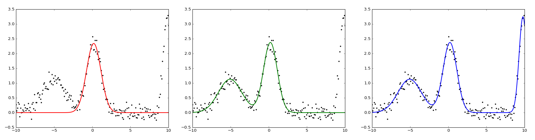
For this example I used curve_fit[4] from the scipy optimization library, which uses a non-linear least squares algorithm. Notice how as I added more Gaussians, the resulting sum became a better approximation of the raw data.
Fitting On a Sphere
So far we’ve been fitting 1D data sets, but the techniques we’re using also work in multiple dimensions. So for instance, let’s say we had a bunch of scattered samples in random directions on a sphere defined by a 2D spherical coordinate system. And let’s say that these samples represent something like…oh I don’t know…the amount of incoming lighting along an infinitesimally narrow ray oriented in that direction. If we take all of these data points and throw some least squares at it, we can end up with a series of N Spherical Gaussians whose sum can serve as an approximation for radiance in any direction on the sphere! We just need our fitting algorithm to spit out the axis, amplitude, and sharpness of each Gaussian, or if we want can fix one of more of the SG parameters ahead of time and only fit the remaining parameters. It should be immediately obvious why this is useful, since a set of SG coefficients can be stored very compactly compared to a gigantic set of radiance samples. Of course if we only use a few Gaussians the resulting approximation will probably lose details from the original radiance function, but this is no different from spherical harmonics or other common techniques for storing approximate representations of radiance or irradiance. Let’s take a look at what a fit actually looks like using an HDR environment map as input data:
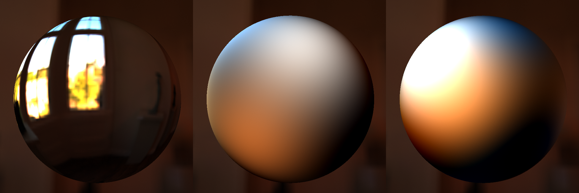
These images were generated Yuriy O’Donnell’s Probulator[5], which is an excellent tool for comparing various ways of approximating radiance and irradiance on a sphere. One important thing to note here is that the fit was only performed on the amplitude of the SG’s: the axis and sharpness are pre-determined based on the number of SG’s. Probulator generates the lobe axis directions using Vogel’s method[6], but any technique for distributing points on a sphere would also work. Fitting only the lobe amplitude significantly simplifies the solve, since there are less parameters to optimize. Solving for a single parameter also allows us to use linear least squares[7], while fitting all of the parameters would require use of complex and expensive non-linear least squares[8] algorithms. Solving for less parameters also decreases the storage costs, since only the amplitudes need to be stored per-probe while the directions and sharpness can be global constants. Either way it’s good to keep in mind when examining the results. In particular it helps explain why the white lobe in the middle image doesn’t quite line up with the bright windows in the source environment. Aside from that, the results are probably what you would expect: doubling the number of lobes increases the possible complexity and sharpness of the resulting approximation, which in this case allows it to provide a better representation of some of the high-frequency details in the source image.
Going Negative
One odd thing you might notice in the SG approximation is the overly dark areas towards the bottom-right of the sphere. They look somewhat similar to the darkening that can show up in SH approximations, which happens due to negative coefficients being used for the SH polynomials. It turns out that something very similar is happening with our SG fit: the least squares optimizations is returning negative coefficients for some of our lobes in an attempt to minimize the error of the resulting fit.If you’re having trouble understanding why this would happen, let’s go back to 1D for a quick example. For the last 1D example I cheated a bit: the data we were fitting our Gaussians to was actually just some random noise applied to the sum of 3 Gaussians. This is why our Gaussian fit so closely resembled the source data. This time, we’ll fitting some lobes to a more complex data set:
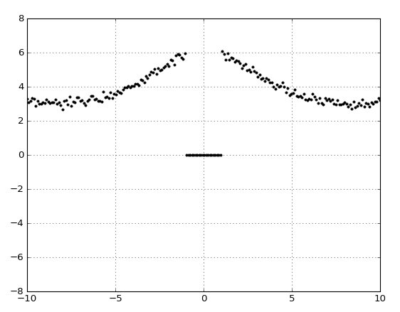
This time the data has a bunch of values near the center that have a value of zero. With such a data set it’s now less obvious how a sum of Gaussians could approximate the values. If we throw least squares at the problem and have it fit two lobes, we get the following:
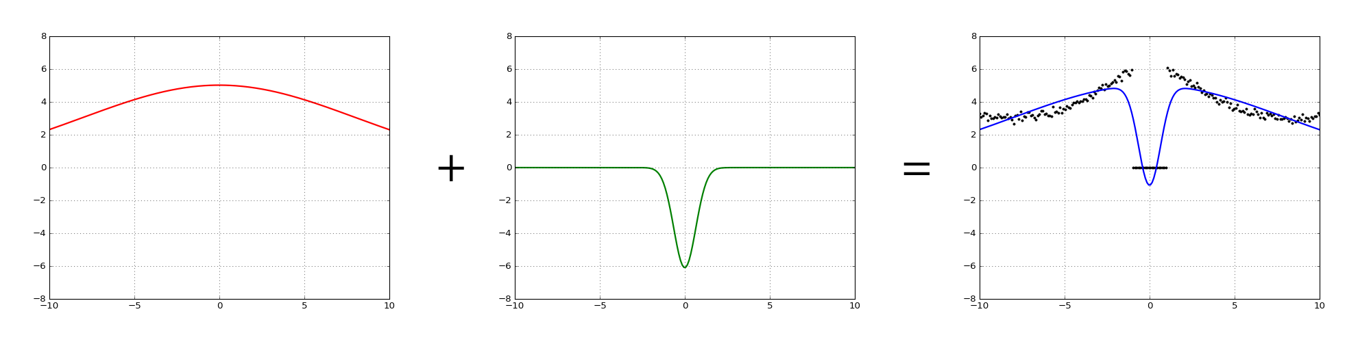
This time around the optimization resulted in a positive amplitude for the first lobe, but a negative amplitude for the second lobe. Looking at the sum overlaid onto to the data makes it clear why this happened: the positive lobe takes care of the all of the positive data points to the left and right, while the negative lobe brings the sum closer to zero in the middle of the graph. Upon closer inspection the negative actually causes the approximation to dip below zero into the negatives. We can assume that having this dip results in lower overall error for the approximation, since that’s how least squares works.
In practice, having negative coefficients and negative values from our approximation can be undesirable. In fact when approximating radiance or irradiance negative values really just don’t make sense, since they’re physically impossible. In our experience we also found that the visual result of lighting a scene with negative lobes can be quite displeasing, since it tends to look very unnatural to have surfaces that are completely dark. Perhaps you remember this image from the first article showing what L2 SH looks like with a bright area light in the environment:

We found that character faces in particular tended to look really bad when our SH light probes had strong negative lobes, and this turned out to be one of our motivations for investigating alternative approximations. We also ran into some trouble when attempting to compress signed floating point values in BC6H textures: some compressors didn’t even support compressing to that format, and those that did had noticeably worse quality.
With that in mind, it would be nice to constrain a least squares solver in such a way that it only gave us positive coefficients. Fortunately for us such a technique exists, and it’s known as non-negative least squares[9] (or NNLS for short). If we use that technique for fitting SG’s to our original radiance function instead of standard least squares, we get this result instead:

This time we don’t have the dark areas in the bottom right, since the fit only uses positive lobes. But unfortunately there’s no free lunch here, since the resulting approximation is also a bit “blurrier” compared to the normal least squares fit.
Comparing Irradiance
Now that we’ve covered how to generate an SG approximation of radiance from source data, we can take a look at how well it stacks up against other options for a simple use case. Probably the most obvious application is computing irradiance from the radiance approximation, which can be directly used to compute standard Lambertian diffuse lighting. The following images were captured using Probulator, and they show the Stanford Bunny being lit using a few common techniques for approximating irradiance:
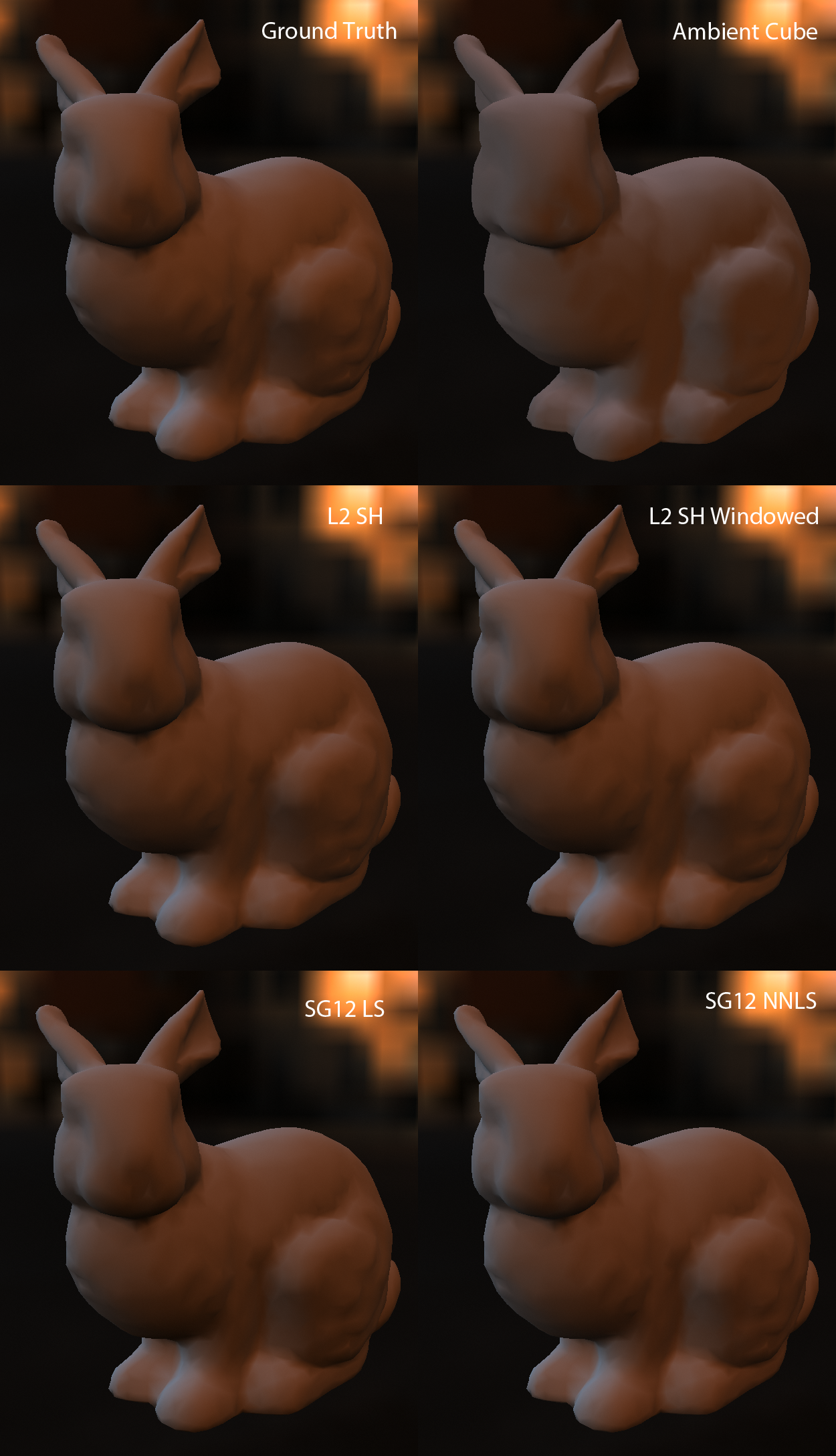
With the exception of Valve’s Ambient Cube, all of the approximations hold up very well when compared with the ground truth. The non-negative least squares fit is just a bit more washed out than the least squares fit, but both seem to produce perfectly acceptable results. The SH result is also very good, with no noticeable ringing artifacts. However this particular environment is a somewhat easier case, as the range of intensities isn’t as large as you might find in some realistic lighting scenarios. For a more extreme case, let’s now look at a comparison using the “Ennis” environment map:
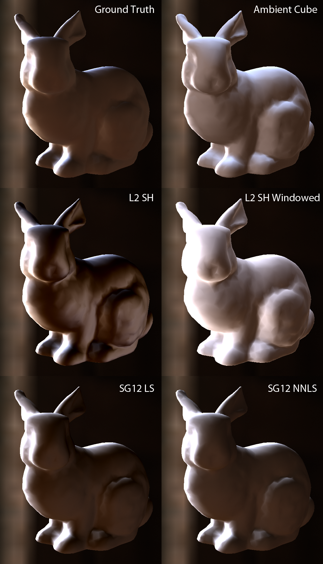
This time there’s a much more noticeable difference between the various techniques. This is because the source environment map has a very bright window to the left, which effectively serves as a large area light source. With this particular environment the SG results start to compare pretty favorably to the SH or ambient cube approximations. The results from L2 SH have severe ringing artifacts, which manifests as areas that are either too dark or too bright on the side of the bunny facing to the right. Meanwhile , the windowed version of L2 SH blurs the lighting too much, making it appear as if the environment is more uniform than it really is. The ambient cube probe doesn’t suffer from ringing, but it does have problems with the bright lighting from the left bleeding onto the top and side of the bunny. Looking at the least squares solve for 12 SG’s, the result is pretty nice but there is a bit of ringing evident on the upper-right side of the bunny model. This ringing isn’t present in the non-negative least squares solve, since all of the coefficients end up being positive.
As I mentioned earlier, these Probulator comparisons use fixed lobe directions and sharpness. Consequently we only need to store amplitude, meaning that the storage cost of the 12 SG lobes is equivalent to 12 sets of floating-point RGB coefficients (36 floats total). L2 SH requires 9 sets of RGB coefficients, which adds up to 27 floats. The ambient cube requires only 6 sets of RGB coefficents, which is half that of the SG solve. So for this particular comparison the SG representation of radiance requires the most storage, however this highlights one of the nice points using SG as your basis: you can solve for any number of lobes you’d like, allowing you to choose easily trade off quality vs. storage and performance cost. Valve’s ambient cube is only defined for 6 lobes, and that number can’t be increased since the lobes must remain orthogonal to each other.
Fitting on a Hemisphere
For full lighting probes where the sampling surface can have any orientation, storing the radiance or irradiance on a sphere makes perfect sense. However it makes less sense if we would like to store baked lighting in 2D textures where all of the sample points lie on the surface of a mesh. For that case storing data for a full sphere is wasteful, since half of the data will point “into” the surface and therefore won’t be useful. With SG’s this is fairly trivial to correct: we can just choose to solve for lobes that only lie on the upper hemisphere surrounding the surface’s normal direction.

To fully generate the compact radiance representation for an entire 2D lightmap, we need to gather radiance samples at every texel location, and then perform a solve to fit the samples to a set of SG lobes. It’s really no different from the spherical probe case we used as a testbed in Probulator, except now we’re generating many probes. The other main differences is that for lightmap generating the appropriate radiance requires sampling a full 3D scene, as opposed to using an environment map as we did with Probulator. This sort of problem is best solved with a ray tracer, using an algorithm such as path tracing to compute the incoming radiance for a particular ray. The following image shows a visualization of what the lightmap result looks like for a simple scene:
Specular
In the previous article we covered techniques that can be used to compute a specular term from SG light sources. If we apply them to a set of lobes that approximate the incoming radiance, then we can compute an approximation of the full environment specular response. For small lobe counts this is only going to be practical for materials with a relatively high roughness. This is because our SG approximation of the incoming radiance won’t be able to capture high-frequency details from the environment, and it would it be very obvious if those details were missing from the reflections on smooth surfaces. However for rougher surfaces where the BRDF itself starts to act as a low-pass filter, an SG approximation won’t have as much noticeable error. As an example, here’s what SG specular looks like for a test scene with a GGX roughness value of 0.25:
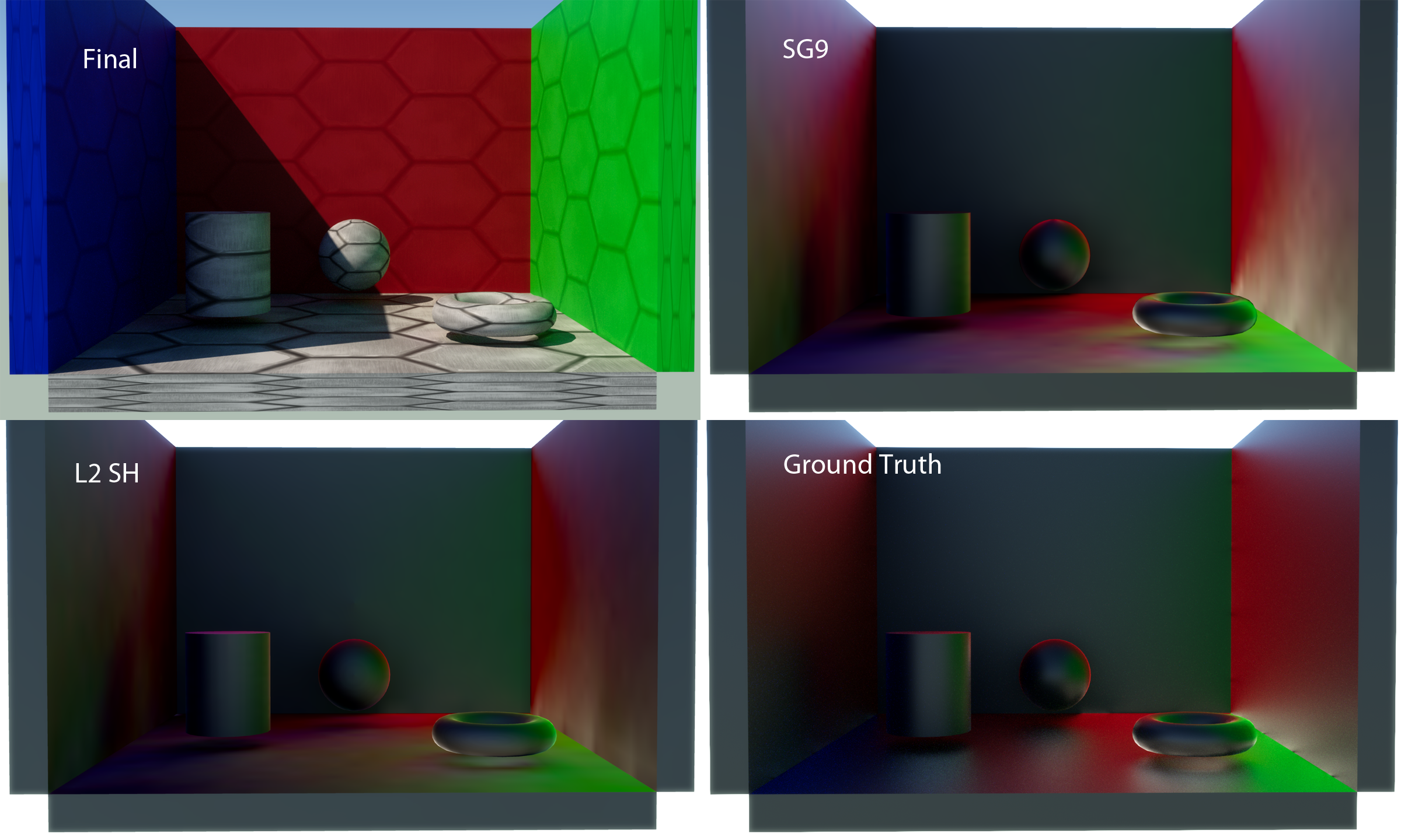
Compared to the ground truth, the SG approximation does pretty well in some places and not-so-well in others. In general it captures a lot of the overall specular response, but suffers from some of the higher-frequency detail being absent in the probes. This results in certain areas looking a bit “washed-out”, such as the right-most wall of the scene. You can also see that the reflections of the cylinder, sphere, and torus are not properly represented in the SG version for the same reason. On the positive side, lightmap samples are pretty dense in terms of their spatial distribution. They’re far more dense than what you typically achieve with sparse cubemap probes placed throughout the scene, which typically suffer from all kinds of occlusion and parallax artifacts. The SG specular also compares pretty favorably to the L2 SH result (despite having the same storage cost), which looks even more washed-out than the SG result. The SH implementation used a 3D lookup texture to store pre-computed SH coefficients, and you can see some interpolation artifacts from this method if you look at the far wall perpendicular to the camera.
Implementation in The Order: 1886
In the first part of our presentation[10] at last year’s Physically Based Shading Course[11], Dave covered some of these details and also shared some information about how we implemented SG lighting probes into The Order: 1886. Much of the implementation was very similar to what I’ve described in this series of articles: we stored 5-12 SG lobes (the count was chosen per-level chunk) in our 2D lightmaps with fixed axis directions and sharpnesses, and we evaluated diffuse and specular lighting using the approximations that I outlined earlier. For dynamic meshes, we baked uniform 3D grids of spherical probes containing 9 SG lobes that were stored in 3D textures. The grids were defined by OBB’s that were hand-placed in the scene by our lighting artists, along with density parameters. In both cases we made use of hardware texture filtering to interpolate between neighboring probes before computing per-pixel lighting.
Much of our implementation closely followed the work of Wang[12] and Xu[13], at least in terms of the techniques used for approximating diffuse and specular lighting from a set of SG lobes. Where our work diverged quite a bit was in the choice to use fixed lobe directions and sharpness values. Both Wang and Xu generated their set of SG lobes by performing a solve on a single environment map, which produced the necessary axis, sharpness, and amplitude parameters. In our case, we always knew that we were going need many probes in order to maintain high-fidelity pre-computed lighting for our scenes. At the time (early 2014) we were already employing 2D lightmaps containing L1 H-basis hemispherical probes (4 coefficients) and 3D grids containing L2 spherical harmonics probes. Both could be quite dense in spatial terms, which allowed capturing important shadowing detail.
To make SG’s work with for these requirements, we had to carefully consider our available trade-offs. After getting a simple test-bed up and running where we could bake 2D lightmaps for a scene, it became quickly apparent that varying the axis directions per-texel wasn’t necessarily the best choice for us. Aside from the obvious issue of requiring more storage space and making the solve more complex and expensive, we also ran into issues resulting from interpolating the axis direction over a surface. The problem is most readily apparent at shadow boundaries: one texel might have visibility of a bright light source which causes a lobe to point in that direction, while its neighboring pixel might have no visibility and thus could end up with a lobe pointing in a completely different direction. The axis would then interpolate between the two directions for pixels between the two texels, which can cause noticeable specular shifting. This isn’t necessarily an unsolvable problem (the Frequency Domain Normal Map Filtering paper[14] extended their EM solver with a term that attempts to align neighboring lobes for coherency), but considering our time and memory constraints it made sense to just sidestep the problem altogether. Ultimately we ended up using fixed lobe directions, using the UV tangent frame as the local coordinate space for lightmap probes. Tangent space is natural for this purpose since it’s Z axis is the surface normal of the mesh, and also because it tends to be continuous over a mesh (you’ll have discontinuities wherever you have UV seams, but artists tend to hide those as best they can anyway). For the 3D probe grids, the directions were in world space for simplicity.
After deciding to fix the lobe directions, we also ultimately decided to go with a fixed sharpness value as well. This of course has the same obvious benefits as fixing the axis direction (less storage, simpler solve), which were definitely appealing. However another motivating factor came from the way were doing our solve. Or rather, our lack of a proper solve. Our early testbed performed all lightmap baking on the CPU, which allowed us to easily integrate packages like Eigen[15] so that we could use a battle-tested least squares solver. However our actual production baking farm at Ready at Dawn uses a Cuda baker that leverages Nvidia’s OptiX library to perform arbitrary ray tracing on a cluster of GPU’s.While Cuda does have optimization libraries that could have achieved what we wanted, we faced a bigger problem: memory. Our baker worked by baking many sample points in parallel on the GPU, with a kernel program that would generate and trace the many rays required for monte carlo integration. When we previously used SH and H-basis this approach worked well: both SH and H-basis are built upon orthogonal basis functions, which allows for continuous integration by projecting each sample onto those basis functions. Gathering thousands of samples per-texel is feasible with this setup, since those samples don’t need to be explicitly stored in memory. Instead, each new sample is projected onto the in-progress result for the texel and then discarded. This is not the case when performing a solve: the solver needs access to all of the samples, which means keeping them all around in memory. This is a big problem when you have many texels in flight simultaneously, and only a limited amount of GPU memory. Like the intepolation issue it’s probably not unsolveable, but we really looking for a less risky approach that would be more of a drop-in replacement for the SH integration.
Ultimately we ended up saying “screw it”, and projected on the SG lobes as they formed an orthogonal basis (even though they didn’t). Since the basis functions weren’t orthogonal the results ended up rather blurry compared to a least squares solve, which muddied some of the detail in the source environment for a probe. Here’s a comparison to show you what I mean:

Of the three techniques presented here, the naive projection is the worst at capturing the details from the source map and also the blurriest. As we saw earlier the least squares solve is the best at capturing sharp changes, but achieves this by over-darkening certain areas. NNLS is the “just right” fit for this particular case, doing a better job of capturing details compared to the projection but without using any negative lobes.
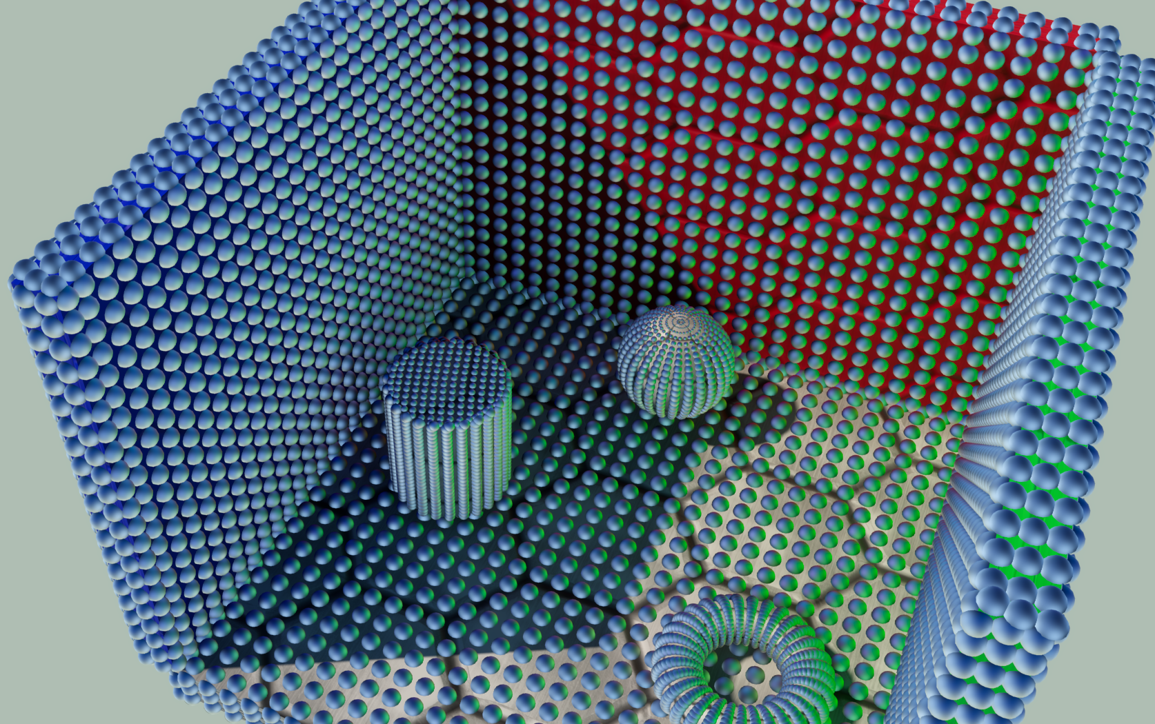
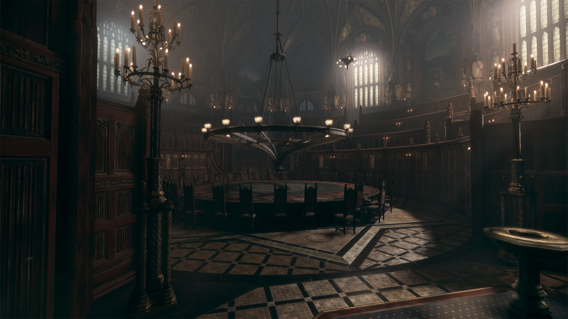
Before we switched to baking SG probes for our grids and lightmaps, we had a fairly standard system for applying pre-convolved cubemap probes that were hand-placed throughout our scenes. Previously these were our only source of environment specular lighting, but once we had SG’s working we began to to use the SG specular approximation to compute environment specular directly from lightmaps and probe grids. Obviously our low number of SG’s was not sufficient for accurately approximating environment specular for smooth and mirror-like surfaces, so our cubemap system remained relevent. We ended up coming up with a simple scheme to choose between cubemap and lightmap specular per-pixel based on the surface roughness, with a small zone in between where we would blend between the two specular sources. The following images taken from our SIGGRAPH slides use a color-coding to showing the specular source chosen for each pixel from one of our scenes:

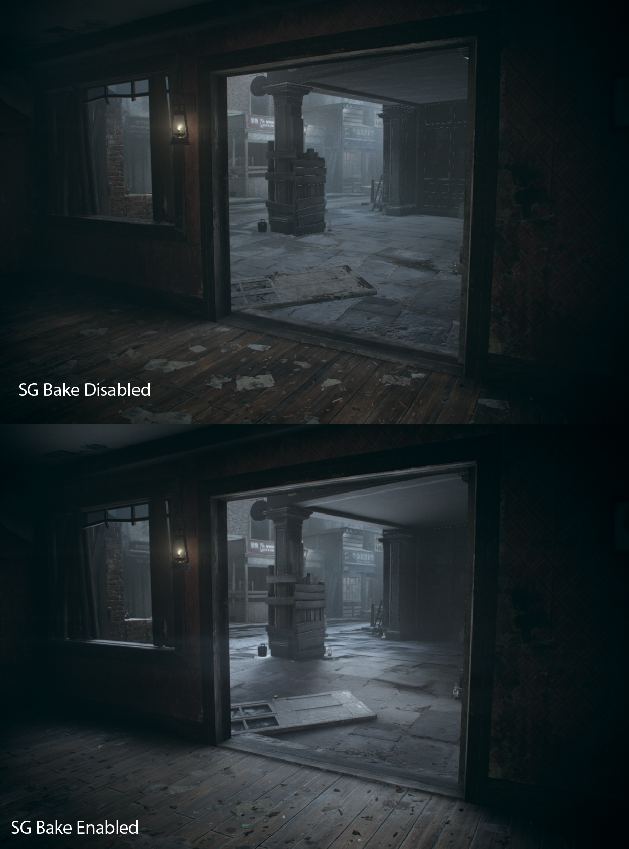
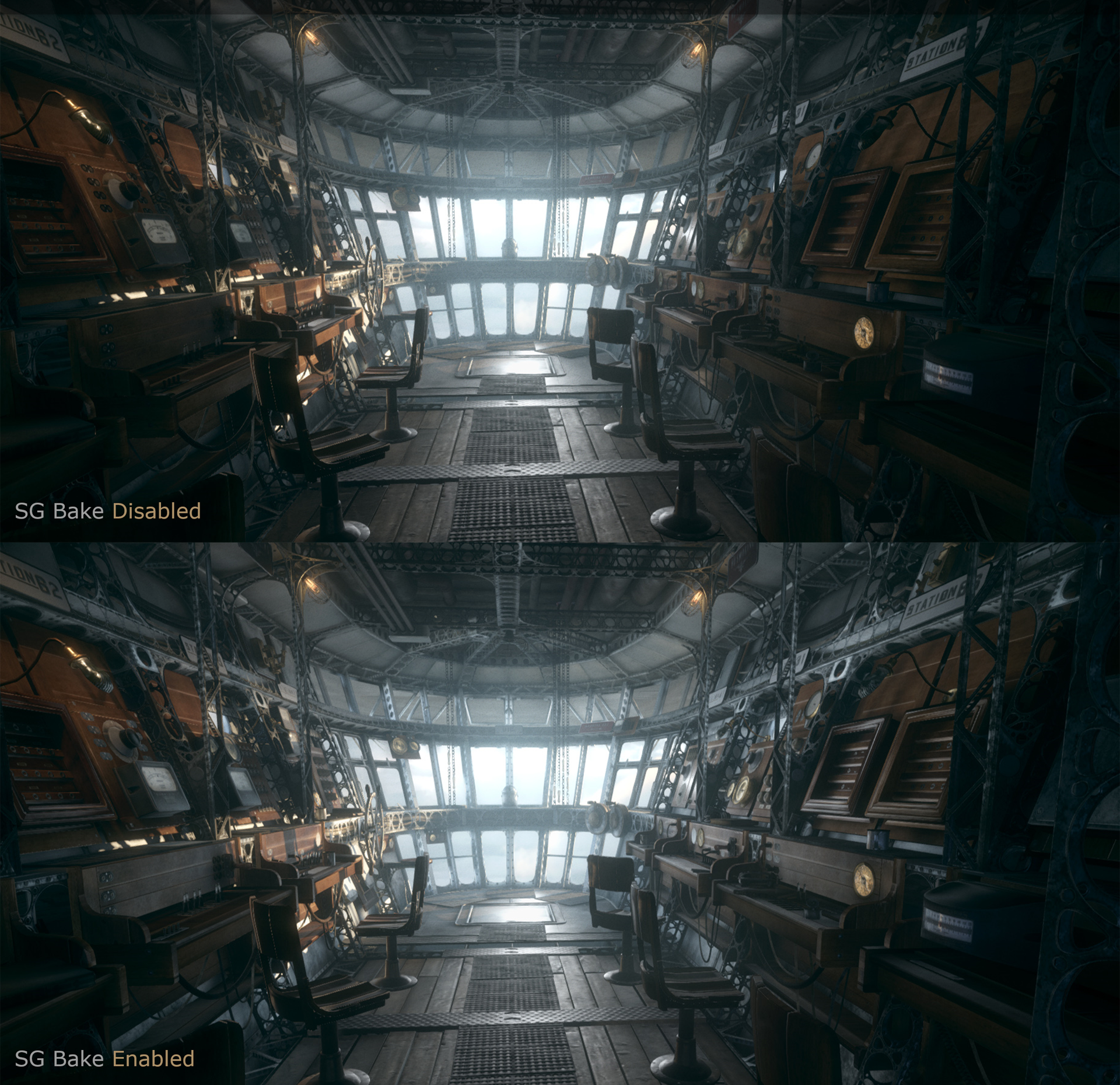
To finish off, here’s some more comparison images taken from our SIGGRAPH slides:

Future Work
We were quite happy with the improvements that come from the SG baking pipeline we introduced for The Order, but we also feel like we’ve barely scratched the surface. Our decision to use fixed lobe directions and sharpness values was probably the right one, but it also limits what we can do. When you take SG’s and compare them to a fixed set of basis functions like SH, perhaps the biggest advantage is the fact that you can use an arbitrary combination of lobes to represent a mix of high and low-frequency features. So for instance you can represent a sun and a sky by having one wide lobe with the sky color, and one very narrow and bright lobe oriented towards the sun. We gave up that flexibility when we decided to go with our simpler ad-hoc projection, and it’s something we’d like to explore further in the future. But until then we can at least enjoy the benefits of having a representation that allows for an environment specular approximation and also avoids ringing artifacts when approximating diffuse lighting.
Aside from the solve, I also think it would be worth taking the time to investigate better approximations for the specular BRDF. In particular I would like to try using something better than just evaluating the cosine, Fresnel, and shadow-masking terms at the center of the warped BRDF lobe. The assumption that those terms are constant over the lobe break down the most when the roughness is high, and in our case we’re only ever using SG specular for rough materials! Therefore I think it would be worth the effort to come up with a more accurate representation of those terms.
References
[1] Curve fitting
[2] Regression analysis
[3] Least squares
[4] scipy.optimize.curve_fit
[5] Probulator
[6] Spreading points on a disc and on a sphere
[7] Linear least squares
[8] Non-linear least squares
[9] Non-negative least squares
[10] Advanced Lighting R&D at Ready At Dawn Studios
[11] SIGGRAPH 2015 Course: Physically Based Shading in Theory and Practice
[12] All-Frequency Rendering of Dynamic, Spatially-Varying Reflectance
[13] Anisotropic Spherical Gaussians
[14] Frequency Domain Normal Map Filtering
[15] Eigen
Comments:
This is so clearly explained that a simple lighting artist like me can finally understand how SH and SG works. thank you!
#### [VisorZ]( "s.pietschmann@campus.tu-berlin.de") -
Thank you very much for the time you’ve put into your explanations. They are a consistent and easy to understand introduction to the usefulness of SHs and SGs.
#### [tomgroveblog](http://tomgroveblog.wordpress.com "tomkelgrove@yahoo.co.uk") -
Excellent series, thanks for posting!