SG Series Part 1: A Brief (and Incomplete) History of Baked Lighting Representations
This is part 1 of a series on Spherical Gaussians and their applications for pre-computed lighting. You can find the other articles here:
Part 1 - A Brief (and Incomplete) History of Baked Lighting Representations
Part 2 - Spherical Gaussians 101
Part 3 - Diffuse Lighting From an SG Light Source
Part 4 - Specular Lighting From an SG Light Source
Part 5 - Approximating Radiance and Irradiance With SG’s
Part 6 - Step Into The Baking Lab
For part 1 of this series, I’m going to provide some background material for our research into Spherical Gaussians. The main purpose is cover some of the alternatives to the approach we used for The Order: 1886, and also to help you understand why we decided to persue Spherical Gaussians. The main empahasis is going to be on discussing what exactly we store in pre-baked lightmaps and probes, and how that data is used to compute diffuse or specular lighting. If you’re already familiar with the concepts of pre-computing radiance or irradiance and approximating them using basis functions like the HL2 basis or Spherical Harmonics, then you will probably want to skip to the next article.
Before we get started, here’s a quick glossary of the terms I use the formulas:
- \( L_{o} \) the outgoing radiance (lighting) towards the viewer
- \( L_{i} \) the incoming radiance (lighting) hitting the surface
- \( \mathbf{o} \) the direction pointing towards the viewer (often denoted as “V” in shader code dealing with lighting)
- \( \mathbf{i} \) the direction pointing towards the incoming radiance hitting the surface (often denoted as “L” in shader code dealing with lighting)
- \( \mathbf{n} \) the direction of the surface normal
- \( \mathbf{x} \) the 3D location of the surface point
- \( \int_{\Omega} \) integral about the hemisphere
- \( \theta_{i} \) the angle between the surface normal and the incoming radiance direction
- \( \theta_{o} \) the angle between the surface normal and the outgoing direction towards the viewer
- \( f() \) the BRDF of the surface
The Olden Days - Storing Irradiance
Games have used pre-computed lightmaps for almost as long as they have been using shaded 3D graphics, and they’re still quite popular in 2016. The idea is simple: pre-compute a lighting value for every texel, then sample those lighting values at runtime to determine the final appearance of a surface. It’s a simple concept to grasp, but there are some details you might not think about if you’re just learning how they work. For instance, what exactly does it mean to store “lighting” in a texture? What exact value are we computing, anyway? In the early days the value fetched from the lightmap was simply multiplied with the material’s diffuse albedo color (typically done with fixed-function texture stages), and then directly output to the screen. Ignoring the issue of gamma correction and sRGB transfer functions for the moment, we can work backwards from this simple description to describe this old-school approach in terms of the rendering equation. This might seem like a bit of a pointless exercise, but I think it helps build a solid base that we can use to discuss more advanced techniques.
So we know that our lightmap contains a single fixed color per-texel, and we apply it the same way regardless of the viewing direction for a given pixel. This implies that we’re using a simple Lambertian diffuse BRDF, since it lacks any sort of view-dependence. Recall that we compute the outgoing radiance for a single point using the following integral:
$$ L_{o}(\mathbf{o}, \mathbf{x}) = \int_{\Omega}f(\mathbf{i}, \mathbf{o}, \mathbf{x}) \cdot L_{i}(\mathbf{i}, \mathbf{x}) \cdot cos(\theta_{i}) \cdot d\Omega $$
If we substitute the standard diffuse BRDF of \( \frac{C_{diffuse}}{\pi} \) for our BRDF (where Cdiffuse is the diffuse albedo of the surface), then we get the following:
$$ L_{o}(\mathbf{o}, \mathbf{x}) = \int_{\Omega} \frac{C_{diffuse}}{\pi} \cdot L_{i}(\mathbf{i}, \mathbf{x}) \cdot cos(\theta_{i}) \cdot d\Omega $$
$$ = \frac{C_{diffuse}}{\pi} \int_{\Omega} L_{i}(\mathbf{i}, \mathbf{x}) \cdot cos(\theta_{i}) \cdot d\Omega $$
On the right side we see that we can pull the constant terms out the integral (the constant term is actually the entire BRDF!), and what we’re left with lines up nicely with how we handle lightmaps: the expensive integral part is pre-computed per-texel, and then the constant term is applied at runtime per-pixel. The “integral part” is actually computing the incident irradiance, which lets us finally identify the quantity being stored in the lightmap: it’s irradiance! In practice however most games would not apply the 1 / π term at runtime, since it would have been impractical to do so. Instead, let’s assume that the 1 / π was “baked” into the lightmap, since it’s constant for all surfaces (unlike the diffuse albedo, which we consider to be spatially varying). In that case, we’re actually storing a reflectance value that takes the BRDF into account. So if we wanted to be precise, we would say that it contains “the diffuse reflectance of a surface with Cdiffuse = 1.0”, AKA the maximum possible outgoing radiance for a surface with a diffuse BRDF.
Light Map: Meet Normal Map
One of the key concepts of lightmapping is the idea of reconstructing the final surface appearance using data that’s stored at different rates in the spatial domain. Or in simpler words, we store lightmaps using one texel density while combining it with albedo maps that have a different (usually higher) density. This lets us retain the appearance of high-frequency details without actually computing irradiance integrals per-pixel. But what if we want to take this concept a step further? What it we also want the irradiance itself to vary in response to texture maps, and not just the diffuse albedo? By the early 2000’s normal maps were starting to see common use for this purpose, however they were generally only used when computing the contribution from punctual light sources. Normal maps were no help with light maps that only stored a single (scaled) irradiance value, which meant that that pure ambient lighting would look very flat compared to areas using dynamic lighting:

To make lightmaps work with normal mapping, we need to stop storing a single value and instead somehow store a distribution of irradiance values for every texel. Normal maps contain a range of normal directions, where those directions are generally restricted to the hemisphere around a point’s surface normal. So if we want our lightmap to store irradiance values for all possible normal map values, then it must contain a distribution of irradiance that’s defined for that same hemisphere. One of the earliest and simplest examples of such a distribution was used by Half-Life 2[1], and was referred to as Radiosity Normal Mapping[2]:
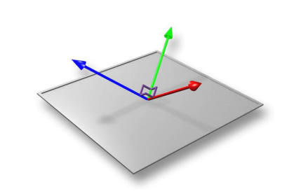
Valve essentially modified their lightmap baker to compute 3 values instead of 1, with each value computed by projecting the irradiance signal onto one of the corresponding orthogonal basis vectors in the above image. At runtime, the irradiance value used for shading would be computed by blending the 3 lightmap values based on the cosine of the angle between the normal map direction and the 3 basis directions (which is cheaply computed using a dot product). This allowed them to effectively vary the irradiance based on the normal map direction, thus avoiding the “flat ambient” problem described above.
While this worked for their static geometry, there still remained the issue of applying pre-computed lighting to dynamic objects and characters. Some early games (such as the original Quake) used tricks like sampling the lightmap value at a character’s feet, and using that value to compute ambient lighting for the entire mesh. Other games didn’t even do that much, and would just apply dynamic lights combined with a global ambient term. Valve decided to take a more sophisticated approach that extended their hemispherical lightmap basis into a full spherical basis formed by 6 orthogonal basis vectors:
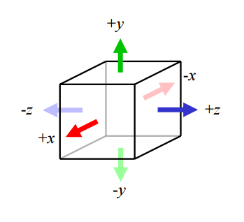
The basis vectors coincided with the 6 face directions of a unit cube, which led Valve to call this basis the “Ambient Cube”. By projecting irradiance in all directions around a point in space (instead of a hemisphere surrounding a surface normal) onto their basis functions, a dynamic mesh could sample irradiance for any normal direction and use it to compute diffuse lighting. This type of representation is often referred to as a lighting probe, or often just “probe” for short.
Going Specular
With Valve’s basis we can combine normal maps and light maps to get diffuse lighting that can vary in response to high-frequency normal maps. So what’s next? For added realism we would ideally like to support more complex BRDF’s, including view-dependent specular BRDF’s. Half-Life 2 handled environment specular by pre-generating cubemaps at hand-placed probe locations, which is still a common approach used by modern games (albeit with the addition of pre-filtering[3] used to approximate the response from a microfacet BRDF). However the large memory footprint of cubemaps limits the practical density of specular probes, which can naturally lead to issues caused by incorrect parallax or disocclusion.
With that in mind it would nice to be able to get some sort of specular response out of our lightmaps, even if only for a subset of materials. But if that is our goal, then our approach of storing an irradiance distribution starts to become a hinderance. Recall from earlier that with a diffuse BRDF we were able to completely pull the BRDF out of the irradiance integral, since the Lambertian diffuse BRDF is just a constant term. This is no longer the case even with a simple specular BRDF, whose value varies depending on both the viewing direction as well as the incident lighting direction.
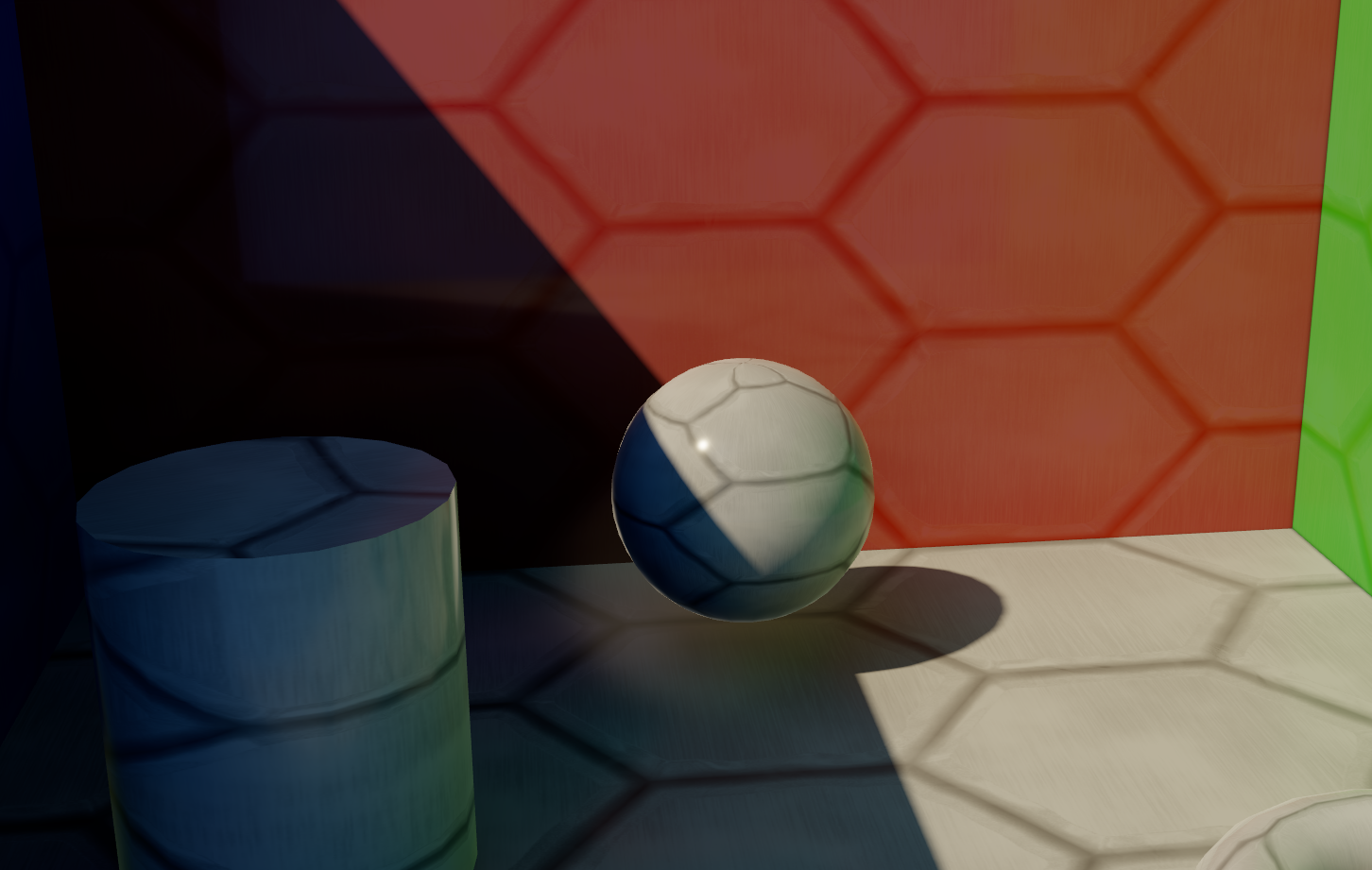
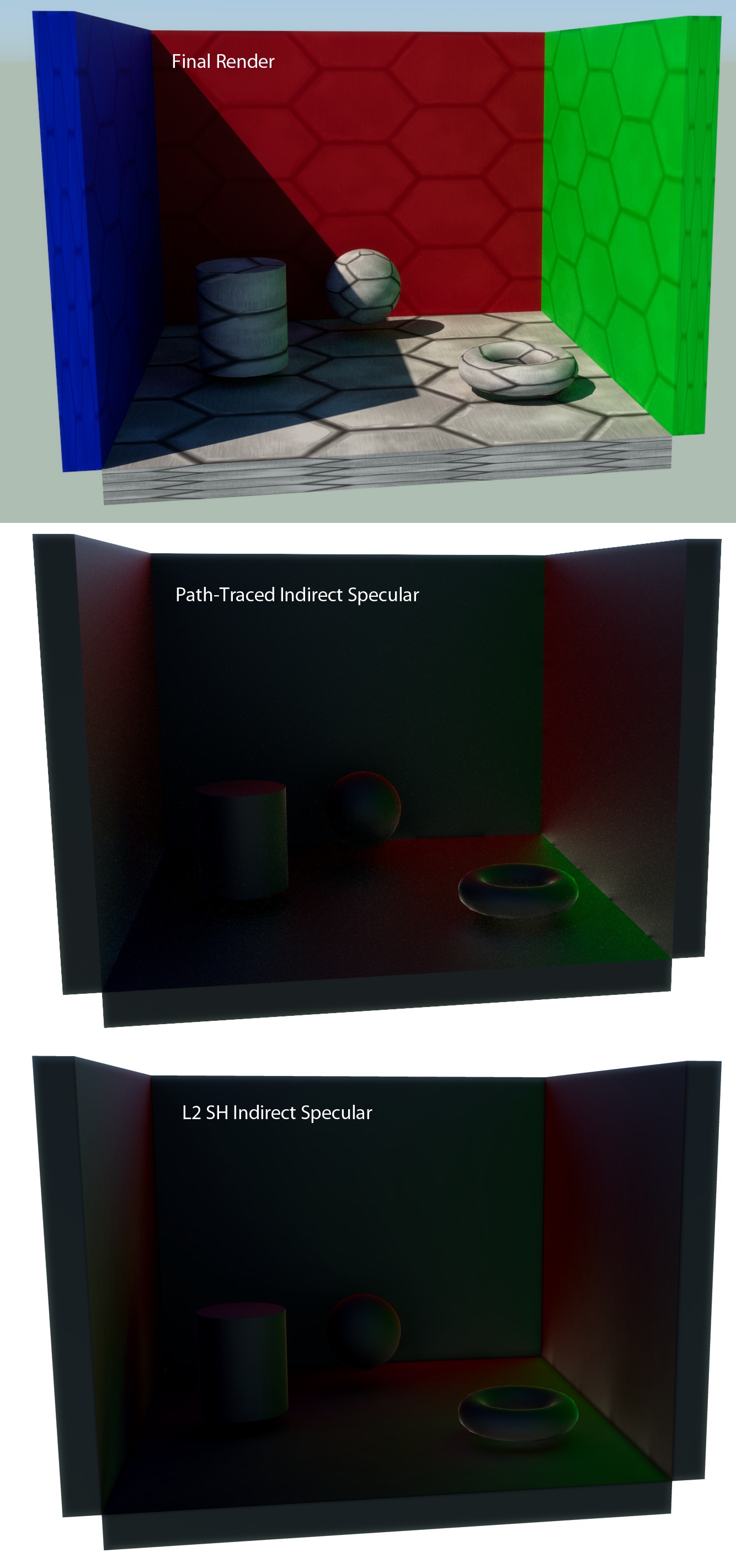
If you’re working with the Half-Life 2 basis (or something similar), a tempting option might be to compute a specular term as if the 3 basis directions were directional lights. If you think about what this means, it’s basically what you get if you decide to say “screw it” and pull the specular BRDF out of the irradiance integral. So instead of Integrate(BRDF * Lighting * cos(theta)), you’re doing BRDF * Integrate(Lighting * cos(theta)). This will definitely give you something, and it’s perhaps a lot better than nothing. But you’ll also effectively lose out on a ton of your specular response, since you’ll only get specular when your viewing direction appropriately lines up with your basis directions according the the BRDF slice. To show you what I mean by this, here’s a comparison:

Hopefully these images clearly show the problem that I’m describing. In the bottom image, you get specular reflections that look just like they came from a few point lights, since that’s effectively what you’re simulating. Meanwhile in the middle image with proper environment reflections, you can see that the the entire green wall effectively acts as an area light, and you get a very broad specular reflections across the entire floor. In general the problem tends to be less noticeable though as roughness increases, since higher roughness naturally results in broader, less-defined reflections that are harder to notice.
Let’s Try Spherical Harmonics
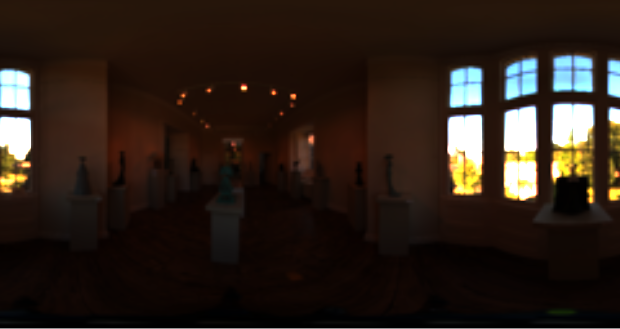
If we want to do better, we must instead find a way to store a radiance distribution and then efficiently integrate it against our BRDF. It’s at this point that we turn to spherical harmonics. Spherical harmonics (SH for short) have become a popular tool for real-time graphics, typically as a way to store an approximation of indirect lighting at discrete probe locations. I’m not going to go into the full specifics of SH since that could easily fill an entire article[4] on its own. If you have no experience with SH, the key thing to know about them is that they basically let you approximate a function defined on a sphere using a handful of coefficients (typically either 4 or 9 floats per RGB channel). It’s sort-of as if you had a compact cubemap, where you can take a direction vector and get back a value associated with that direction. The big catch is that you can only represent very low-frequency (fuzzy) signals with lower-order SH, which can limit what sort of things you can do with it. You can project detailed, high-frequency signals onto SH if you want to, but the resulting projection will be very blurry. Here’s an example showing what an HDR environment map looks like projected onto L2 SH, which requires 27 coefficients for RGB:

In the case of irradiance, SH can work pretty well since it’s naturally low-frequency. The integration of incoming radiance against the cosine term effectively acts as a low-pass filter, which makes it a suitable candidate for approximation with SH. So if we project irradiance onto SH for every probe location or lightmap texel, we can now do an SH “lookup” (which is basically a few computations followed by a dot product with the coefficients) to get the irradiance in any direction on the sphere. This means we can get spatial variation from albedo and normal maps just like with the HL2 basis!
It also turns out that SH is pretty useful for computing irradiance from input radiance, since we can do it really cheaply. In fact it can do it so cheaply, it can be done at runtime by folding it into the SH lookup process. The reason it’s so cheap is because SH is effectively a frequency-domain representation of the signal, and when you’re in the frequency domain convolutions can be done with simple multiplication. In the spatial domain, convolution with a cubemap is an N^2 operation involving many samples from an input radiance cubemap. If you’re interested in the full details, the process was described in Ravi Ramamoorthi’s seminal paper[5] from 2001, with derivations provided in another article[6].

So we’ve established that SH works for approximating irradiance, and that we can convert from radiance to irradiance at runtime. But what does this have to do with specular? By storing an approximation of radiance instead of irradiance in our probes or lightmaps (albeit, a very blurry version of radiance), we now have the signal that we need to integrate our specular BRDF against in order to produce specular reflections. All we need is an SH representation of our BRDF, and we’re a dot product away from environment specular! The only problem we have to solve is how to actually get an SH representation of our BRDF.
Unfortunately a microfacet specular BRDF is quite a bit more complicated than a Lambertian diffuse BRDF, which makes our lives more difficult. For diffuse lighting we only needed to worry about the cosine lobe, which has the same shape regardless of the material or viewing direction. However a specular lobe will vary in shape and intensity depending on the viewing direction, material roughness, and the fresnel term at zero incidence (AKA F0). If all else fails, we can always use monte-carlo techniques to pre-compute the coefficients and store the result in a lookup texture. At first it may seem like we need at parameterize our lookup table on 4 terms, since the viewing direction is two-dimensional. However we can drop a dimension if we follow in the footsteps[7] of the intrepid engineers at Bungie, who used a neat trick for their SH specular implementation in Halo 3[8]. The key insight that they shared was that the specular lobe shape doesn’t actually change as the viewer rotates around the local Z axis of the shading point (AKA the surface normal). It actually only changes based on the viewing angle, which is the angle between the view vector and the local Z axis of the surface. If we exploit this knowledge, we can pre-compute the coefficients for the set of possible viewing directions that are aligned with the local X axis. Then at runtime, we can rotate the coefficients so that the resulting lobe lines up with the actual viewing direction. Here’s an image to show you what I mean:
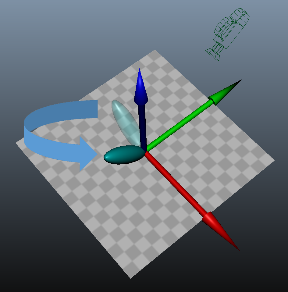
So in this image the checkerboard is the surface being shaded, and the red, green and blue arrows are the local X, Y, and Z axes of the surface. The transparent lobe represents the specular lobe that we precomputed for a viewpoint that’s aligned with the X axis, but has the same viewing angle. The blue arrow shows how we can rotate the specular lobe from its original position to the actual position of the lobe based on the current viewing position, giving us the desired specular response. Here’s a comparison showing what it looks like it in action:
Not too bad, eh? Or at least…not too bad as long as we’re willing to store 27 coefficients per lightmap texel, and we’re only concerned with rough materials. The comparison image used a GGX α parameter of 0.39, which is fairly rough.
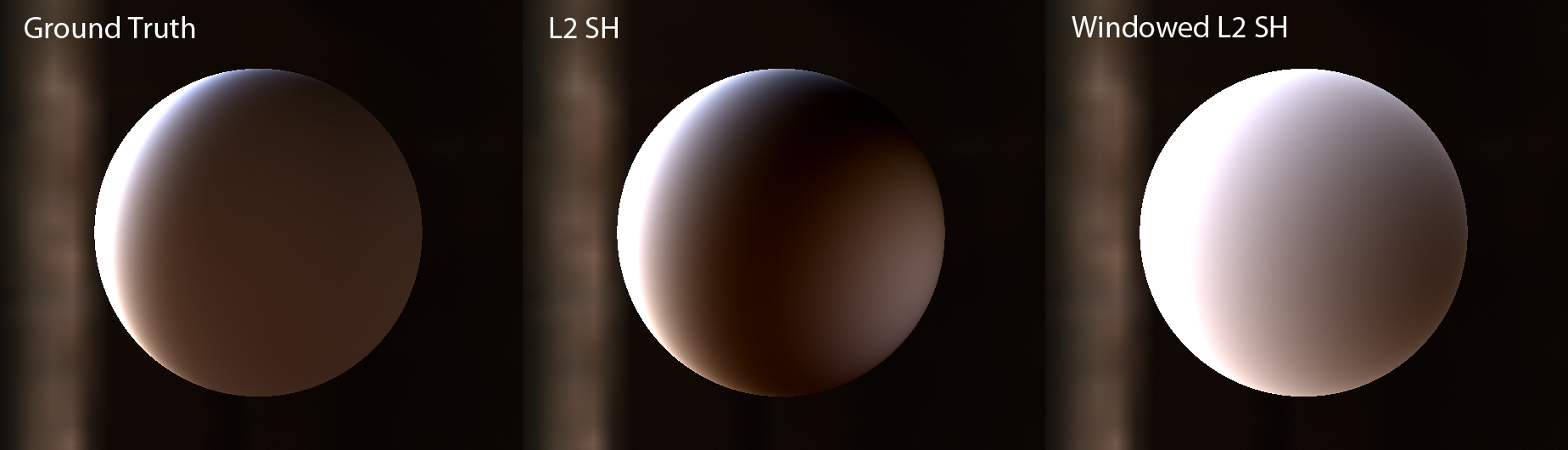
One common issue with issue with SH is a phenomenon known as “ringing”, which is described in Peter-Pike Sloan’s Stupid Spherical Harmonics Tricks[9]. Ringing artifacts tends to show up when you have a very intense light source one side of the sphere. When this happens, the SH projection will naturally result in negative lobes on the opposite side of the sphere, whi
h an result very low (or even negative!) values when evaluated. It’s generally not too much of an issue for 2D lightmaps, since lightmaps are only concerned with the incoming radiance for a hemisphere surrounding the surface normal. However they often show up in probes, which store radiance or irradiance about the entire sphere. The solution suggested by Peter-Pike Sloan is to apply a windowing function to the SH coefficients, which will filter out the ringing artifacts. However the windowing will also introduce additional blurring, which may remove high-frequency components from the original signal being projected. The following image shows how ringing artifacts manifest when using SH to compute irradiance from an environment with a bright area light, and also shows how windowing affects the final result:
Update 8/6/2019: For L1 (2-band SH), Graham Hazel developed a technique for Geomerics that reconstructions irradiance from radiance with less ringing and better contrast compared with the process originally developed by Ravi Ramamoorthi. The slides from his presentation have disappeared from the Geomerics website, but you can find the archived version here. You can also find a reference implementation in Yuriy O’Donnell’s Probulator code.
References
[1] Shading in Valve’s Source Engine (SIGGRAPH 2006)
[2] Half Life 2 / Valve Source Shading
[3] Real Shading in Unreal Engine 4
[4] Spherical Harmonic Lighting: The Gritty Details
[5] An Efficient Representation for Irradiance Environment Maps
[6] On the Relationship between Radiance and Irradiance: Determining the illumination from images of a convex Lambertian object
[7] The Lighting and Material of Halo 3 (Slides)
[8] The Lighting and Material of Halo 3 (Course Notes)
[9] Stupid Spherical Harmonics Tricks
Comments:
fang -
Hello! Thank you for sharing such great article. I have a question here. How do you think about vertex baking and texel baking? Why nowadays people tend to use texel baking instead of vertex baking?
### [MJP](http://mynameismjp.wordpress.com/ "mpettineo@gmail.com") -
Hey Tyler, for the bunny image I used the “wells” environment in probulator, which doesn’t have as high of a dynamic range as the “ennis” probe. With the “wells” probe the ringing isn’t particularly noticeable, so I used the standard L2 SH approach with no windowing.
### [MJP](http://mynameismjp.wordpress.com/ "mpettineo@gmail.com") -
There are pros and cons to either approach. Vertex baking tends to be easier to start with since you already have the structure set up for you, and there’s no need to generate a unique 2D parameterization of your entire scene. However the major downside is that your sample density is effectively tied to your vertex density and topology. This means that meshes may need to be tessellated in order to capture high-frequency lighting changes, which can increase vertex, geometry, and pixel costs. With lightmaps the texel density can be adjusted independently of the underlying geometry, which makes it much easier spot fix problem areas. In our studio this was actually very important, since it removed a dependency between the lighting artists and environment artists. The structured 2D layout of textures also tends to be much better for interpolation and compression. On recent hardware you can use block compression formats like BC6H to drastically reduce the memory footprint, which is of course a huge win if you’re memory constrained. Personally I keep a close eye on papers that presentations that look into alternative forms of storing baked sample points for a scene. For instance there are some presentations that have discussed using a sparse 3D grid to store data without needing vertices or 2D maps, and others that have used basis functions to “splat” the contribution of arbitrary points onto a scene.
### [Tayfun K. (@notCamelCase)](http://twitter.com/notCamelCase "notCamelCase@twitter.example.com") -
Very informative posts, thank you! Shouldn’t this be the ‘middle image’ below in comparison of indirect speculars? “Meanwhile in the bottom image with proper environment reflections, you can see that the the entire green wall effectively acts as an area light …”
### [Tyler]( "tylerrobertsondeveloper@gmail.com") -
It’’s difficult to tell, is the source IBL bright enough for the ringing artifact visible on the test with the bunny? Or did you use the windowed L2 SH there?
### [MJP](http://mynameismjp.wordpress.com/ "mpettineo@gmail.com") -
Indeed, that’s exactly right: your normal maps are typically going to be much higher density than your light maps, since normal maps can be tiled and light maps will be completely unique over all surfaces (plus the lightmaps may have a larger per-texel footprint if they are HDR). So technically you *could* sample the normal maps when baking the lightmap, but since the texel density is much lower it would be as if you used a blurrier, downscaled version of the normal map.
### [atrix256]( "alan.wolfe@gmail.com") -
Apologies, I get it now. The normals can’t be taken into consideration because the light map is much lower resolution than the details needed to support features at the normal map level. Thanks for writing these, they are a great read (:
### [atrix256]( "alan.wolfe@gmail.com") -
Hello! For the case of ambient lighting looking flat even in presence of a normal map, near the top of the article, why wasn’t the normal map considered when calculating the baked lighting? It seems like that would also solve the problem, unless there is some reason that is undesirable?
### [MJP](http://mynameismjp.wordpress.com/ "mpettineo@gmail.com") -
Yes you’re 100% correct: that sentence is referring to the middle image, not the bottom image. It’s now been corrected. Thank you for pointing out the mistake!