Breaking Down Barriers - Part 3: Multiple Command Processors

This is Part 3 of a series about GPU synchronization and preemption. You can find the other articles here:

Part 1 - What’s a Barrier?
Part 2 - Synchronizing GPU Threads
Part 3 - Multiple Command Processors
Part 4 - GPU Preemption
Part 5 - Back To The Real World
Part 6 - Experimenting With Overlap and Preemption

Welcome to Part 3 of the series! In this article, I’m going to talk a bit about how multiple command processors can be used to increase the overall performance of a GPU by reducing the amount of time that shader cores sit idle.

Flushing Performance Down The Drain

Looking back on our fictional GPU that we discussed in Part 2, it’s fair to say to its synchronization capabilities are sufficient to obtain correct results from a sequence of compute jobs with coarse-grained dependencies between those jobs. However, the tool that we used to resolve those dependencies (a global GPU-wide barrier that forces all pending threads to finish executing, also known as a “flush”) is a very blunt instrument. It’s bad enough that we’re unable to represent dependencies at the sub-dispatch level (in other words, only some of threads from one dispatch depend on only some of threads from another dispatch), but it can also force us into situations where non-dependent dispatches still can’t overlap with other. This can be really bad when you’re talking about GPU’s that require thousands of threads to fill all of their executions units, particularly if your dispatches tend towards low thread counts and high execution times. If you recall from Part 2, we discovered that the cost of each GPU-wide barrier was tied to the corresponding decrease in utilization, and long-running threads can result in cores sitting idle for a long period of time.

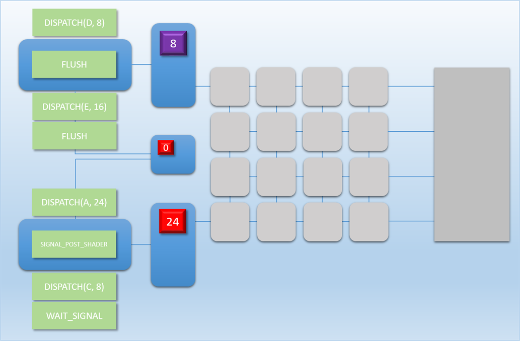
In Part 2 we did discuss one way that the MJP-3000 could extract some extra overlap from a sequence of dispatches. Specifically, we talked about a case with two dependent dispatches, and a third dispatch that was independent of the first two.  By splitting the barrier into two steps ( SIGNAL_POST_SHADER and WAIT_SIGNAL), we could effectively sync only a single dispatch’s threads instead of waiting for all executing threads to finish. It worked in that case, but it’s still very limited tool. In that example we relied on our advance knowledge of dispatch C’s thread count and execution time to set up the command buffer in a way that would maximize overlap. But this may not be practical in the real-world, where thread count and execution time might vary from frame-to-frame. That technique also doesn’t scale up to more complex dependency graphs, since we’re always going to be limited by the fact that there’s only 1 command processor that can wait for something to finish, and then kick off more threads.

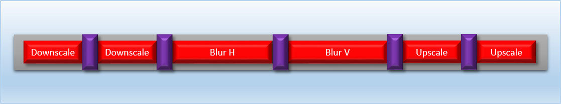
To give you a better idea of what I’m talking about, let’s switch to an example that’s more grounded in reality. In real engines performing graphics work on GPU’s, it’s very common to have chains of draws or dispatches where each one depends on the previous step. For instance, imagine a bloom pass that requires several downsampling steps, followed by several blur passes, followed by several upscale passes. So you might end up with around 6-8 different dispatches, with a barrier between each one:

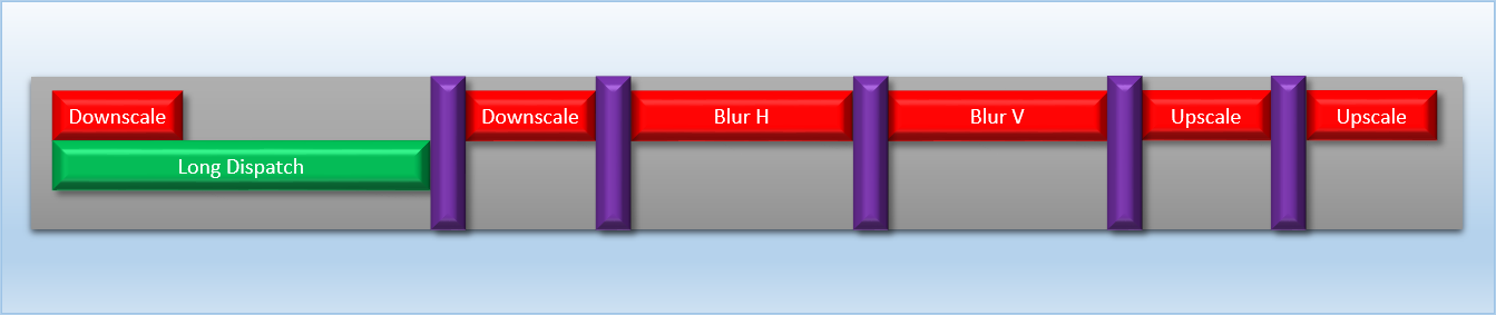
Now, let’s say we would like to overlap this with a large dispatch that takes about an equal amount of time. Overlapping it with a single step is pretty simple: we just need to make sure that a bloom dispatch and the large dispatch end up on the same side of a barrier, and they will overlap with each other. So for instance we could dispatch the large shader, then dispatch the first downscale, and then issue a barrier. However, this might not be ideal if the GPU has a setup similar to our fictional GPU, where our barriers are implemented in terms of commands that require waiting for all previously-launched shaders to finish executing. If  that’s the case, then the first barrier after the long dispatch might cause a long period with no overlap:

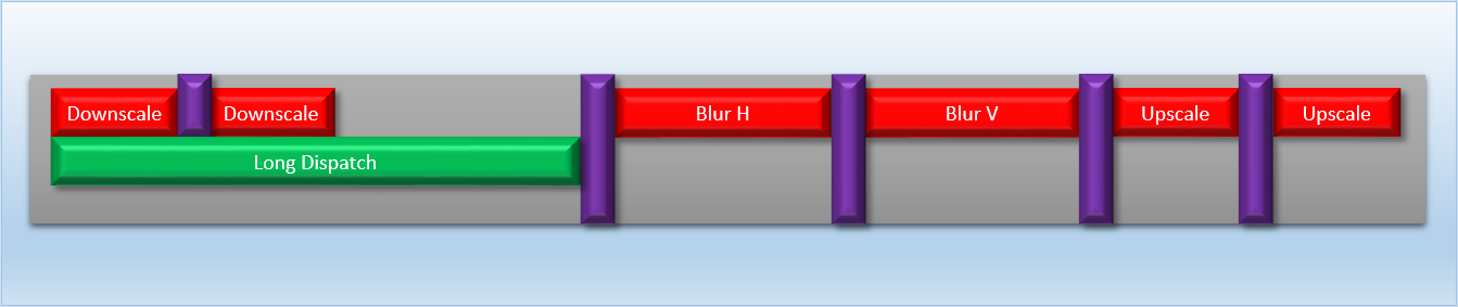
This is better than nothing, but not great. Really we want the long dispatch to fully overlap one of the barriers, since the associated cache flushes and other actions are periods where the shader units would otherwise be completely idle. We can achieve this with split barriers, but we could only do this once if our SIGNAL_POST_SHADER instruction is limited to signaling after all previously-queued threads have completed:

Things could get even more complicated if we wanted to overlap our bloom with a different chain of dispatches. For example, we might have a depth of field technique that needs 4-5 dispatches that are all dependent on the previous dispatch, but are otherwise independent from the bloom dispatches. By interleaving the dispatches from both techniques it would be possible to achieve some overlap, but it would be complex and difficult to balance. In both cases we’re really being held back by the limitations of our barrier implementation, and our lives would be much easier if we could submit each pass as a set of completely independent commands that aren’t affected by each other’s sync operations.

Two Command Processors Are Better Than One

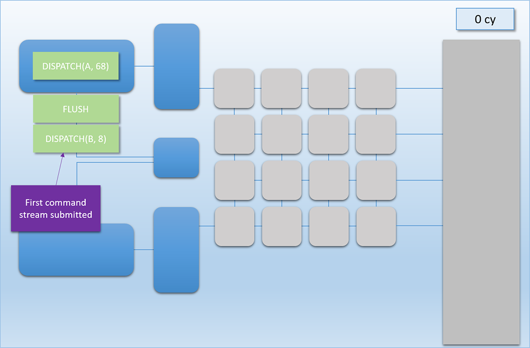
After much, much complaining from the programmers writing software for the MJP-3000 about how much performance they were losing to sync points, the hardware engineers at MJP Industries finally had enough. When designing the all-new MJP-4000, they decided that the simplest way to handle multiple independent command streams would be to go ahead and copy/paste the front-end of the GPU! The logical hardware layout now looks like this:

As you can see, there’s now two command processors attached to two separate thread queues. This naturally gives the hardware the ability to handle two command buffers at once, with two different processors available for performing the flush/wait operations required for synchronization. The MJP-4000 still has the same number of shader cores as the 3000 (16), which means we haven’t actually increased the theoretical maximum throughput of the GPU. However the idea is that by using dual command processors we can reduce the amount of time that those shader cores sit idle, therefore improving the overall throughput of the jobs that it runs.

Looking at the diagram, you might (rightfully) wonder “how exactly do the two front-ends share the shader cores?” On real GPU’s there are several possible ways to handle that, which we will touch on a bit in a later article. But for now, let’s assume that the dual thread queues use a very simple scheme for sharing the cores:

• If only one queue has pending threads and there are any empty shader cores, the queue will fill up those cores with work until there are no cores left

• If both queues have work to do and there are empty cores, those cores are split up evenly and assigned threads from both thread queues (if there’s an odd number of cores available, the top queue gets the extra core)

• Threads always run to completion once assigned to a shader core, which means pending threads can’t interrupt them

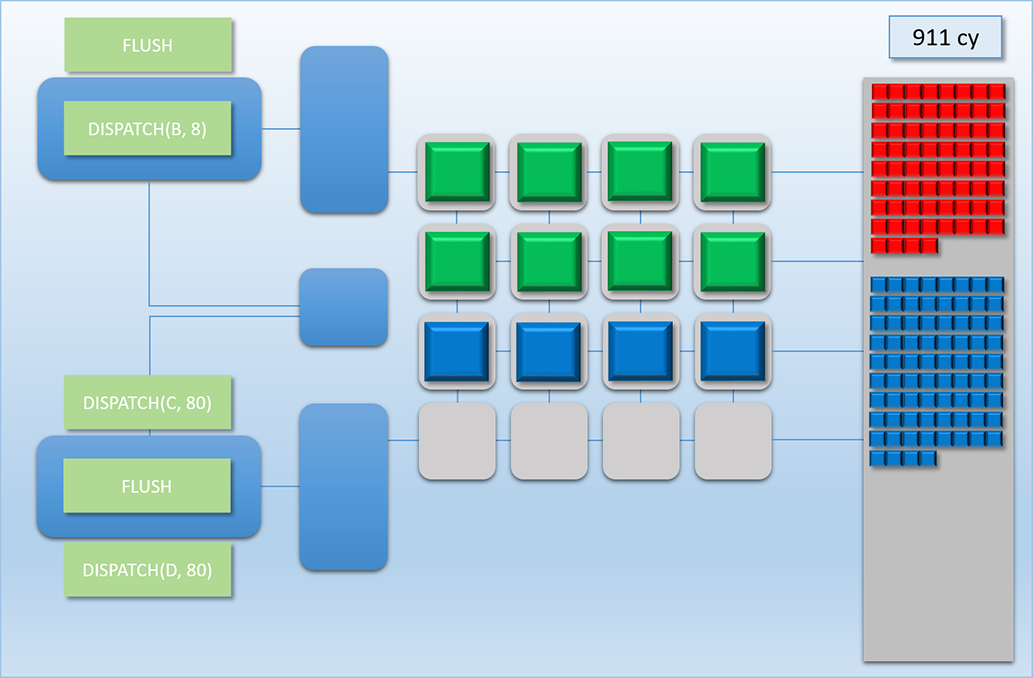
Let’s now look at how all of this all would work out in practice. Let’s imagine we have two independent chains of dispatches to run on the GPU at roughly the same time. Chain 1 consists of two dependent dispatches, which we’ll call Dispatch A (red) and Dispatch B (green). Dispatch A consists of 68 threads that each take 100 cycles to complete. Dispatch B then reads the results of Dispatch A, which means Chain 1 will need a FLUSH command between Dispatch A and Dispatch B. Once the flush completes, Dispatch B then launches another 8 threads that take 400 cycles to complete. Chain 2 also consists of two dependent dispatches, which we’ll call Dispatch C (blue) and Dispatch D (purple). Dispatch C will launch 80 threads that take 100 cycles to complete, followed by another 80 threads that take 100 cycles to complete. Here’s how it plays out:

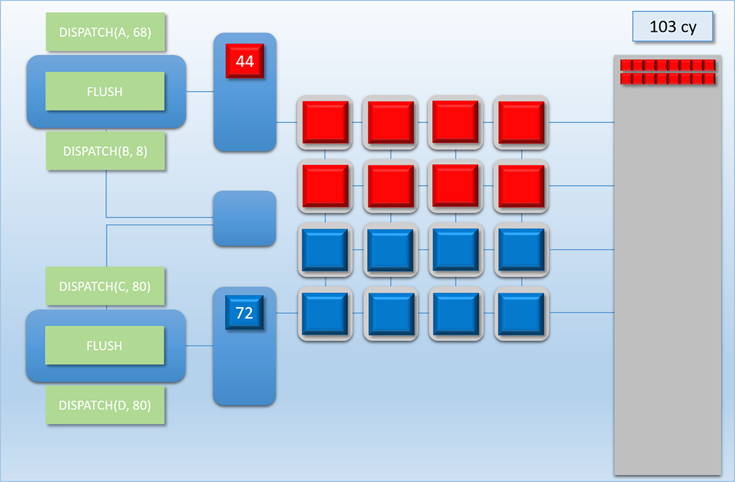
This sequence is easily the most complex example that we’ve looked at, so let’s break it down step by step:

• At cycle 0, we see that Chain 1’s command buffer has been submitted to the top-most command processor, which is ready to execute the Dispatch A command.

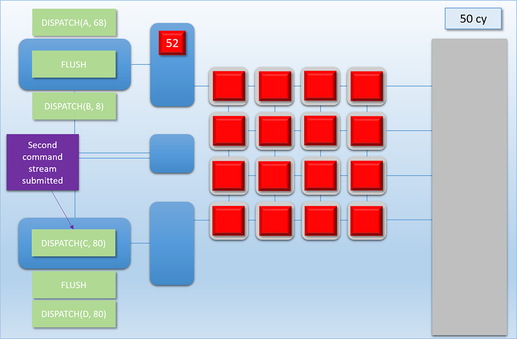
• Next we fast-forward to 50 cycles later, where we see that Dispatch A’s threads have been pushed to the top thread queue, and 16 threads are already running on the shader cores. It’s at this point that Chain 2’s command buffer is submitted to the bottom command processor, with the first command to be processed is Dispatch C.

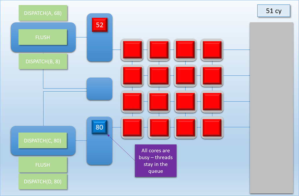
• 1 cycle later at cycle 51, Dispatch C’s threads are sitting in the thread queue, but none of them are actually executing. This is because our all of the shader cores are already busy, and we’ve already stated that our GPU doesn’t interrupt running threads.

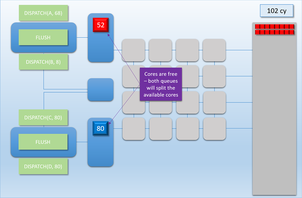
• The 80 threads from Dispatch C need to wait until cycle 102, which is when Dispatch A has written its results to memory and the shader cores are finally freed up.

• 1 cycle later in cycle 103 the two thread queues will evenly split the available cores, and 8 threads from both A and C get assigned to the shader cores. Once we’ve hit this point, the two dispatches continue to evenly share the available cores (since every batch of 8 threads starts and finishes at the same time as the other dispatch’s batch), which continues for about another 500 cycles.

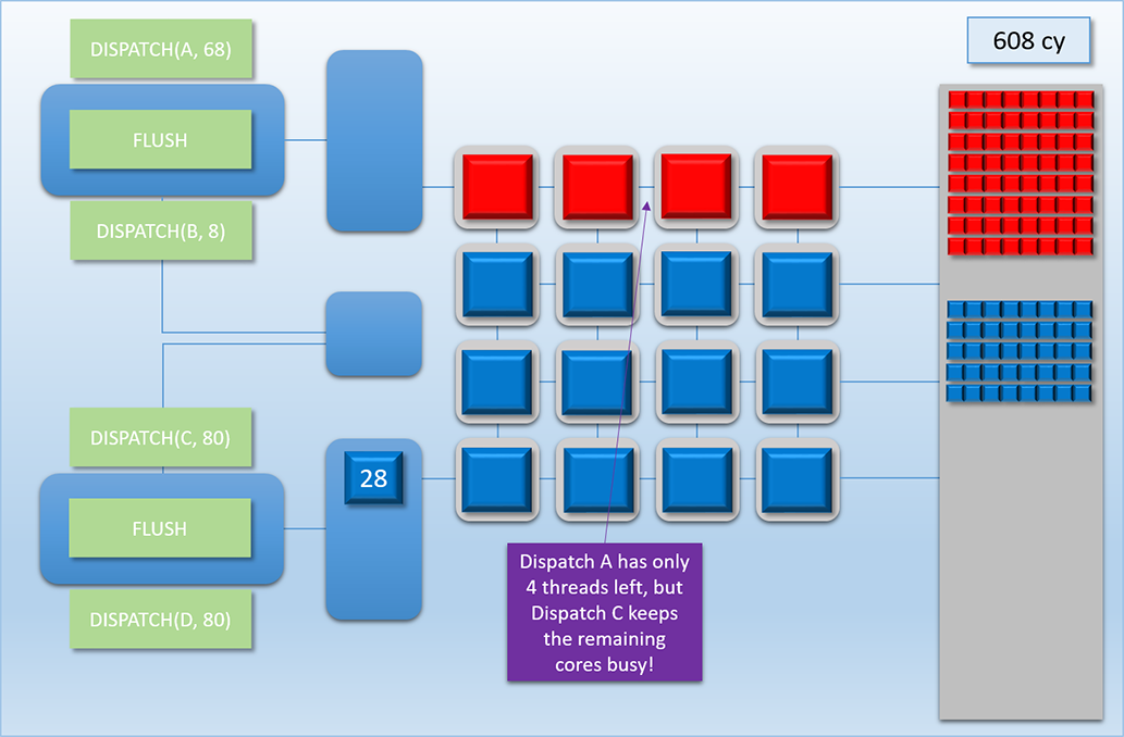
• At cycle 608, something interesting happens. At this point only 4 threads from Dispatch A were running, since that’s all that was left after executing the previous 64 threads. The top-most command processor is running a FLUSH command, which means it’s waiting for those 4 threads to complete before it moves on and executes the next DISPATCH command. This means that if we didn’t have the second command processor + thread queue launching threads from Dispatch C, then 12 of those 16 shader cores would have been idle due to the FLUSH! However by utilizing our dual command buffers, we’ve ensured that those idle cores stay busy with work from another chain!

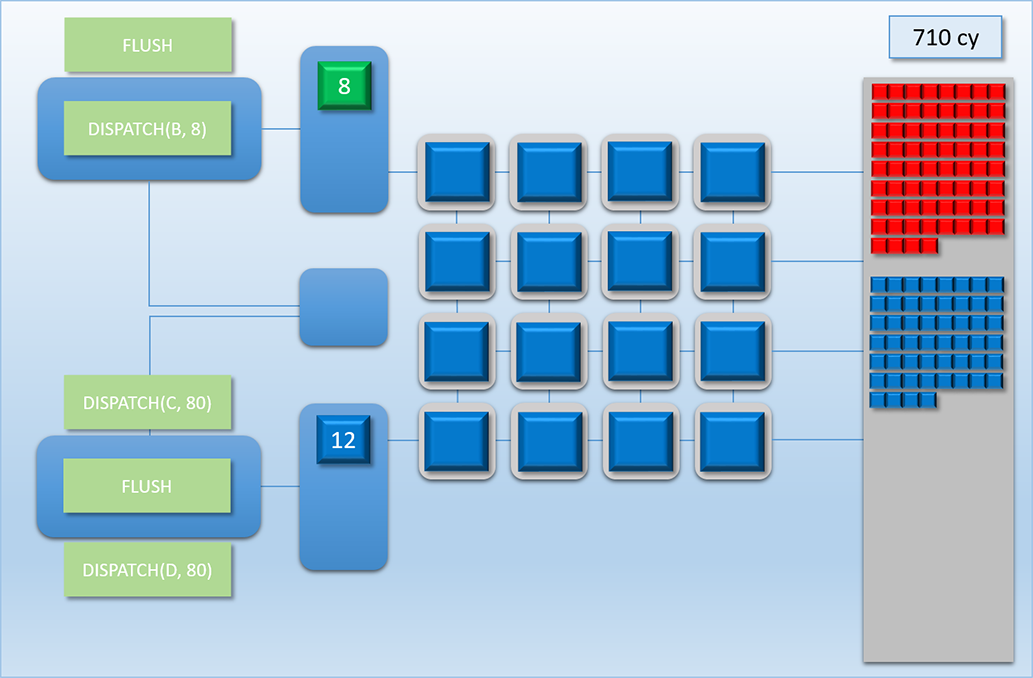
• Moving on to cycle 710, Dispatch A finally finishes writing its results, and Dispatch B gets its 8 threads enqueued in the top-most thread queue. Unfortunately those 8 threads have to wait about 100 cycles for a batch of Dispatch C’s threads to finish, since the bottom thread queue managed to get in there and hog all of the shader cores while the top-most command processor was handing the FLUSH and DISPATCH commands.

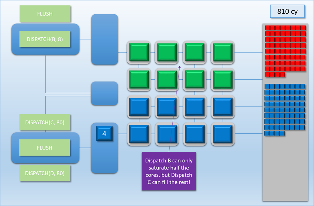
• At cycle 810 things return back to what we had before: both thread queues sharing the shader cores evenly. It should be noted that this is another point where we would normally have idle cores if we didn’t have dual front-ends, since Dispatch B only launched 8 threads! This case is actually even worse than what we had earlier with idle cores being caused by a FLUSH, since threads from Dispatch B take 400 cycles to complete. So it’s a good thing we have that extra front-end!

• At cycle 911 Dispatch C finally starts to wind down, which cause a period of 100 cycles where 4 cores are idle. But of course 100 cycles at 75% utilization is still a lot better than 400 cycles with 50% utilization, so that’s really not so bad.

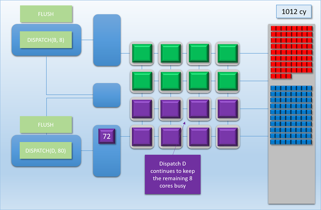
• Around 100 cycles later we hit cycle 1012, where Dispatch D rolls in to once again fill up those remaining 8 shader cores.

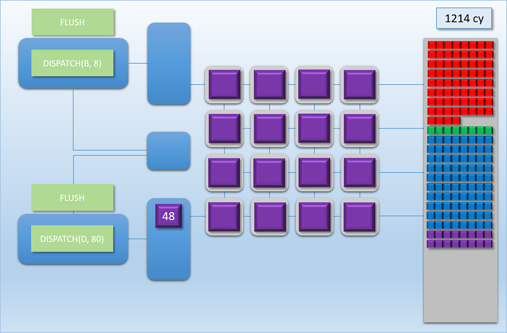
• The sharing continues for about another 200 cycles until Dispatch B finishes at cycle 1214, at which point Dispatch D is free to use all of the cores it wants.

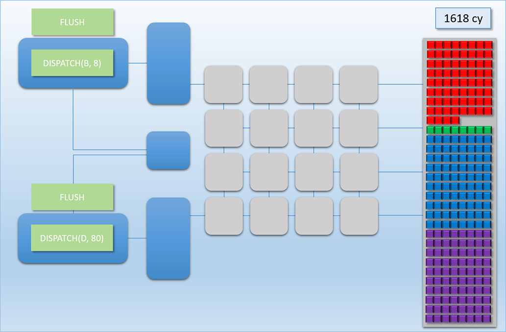
• Finally, at cycle 1618 the last batch from Dispatch D finishes, and all of our results are in memory.

Whew, we made it! The details were a bit complex, but we can distill this down to something much simpler: by executing two command buffers at once, we got an overall higher utilization compared to if we ran them one at a time. Pretty neat, right? However, this higher utilization came at the cost of higher latency for each individual chain. This is similar to what we saw in Part 2 when we overlapped multiple dispatches: it took longer for each separate chain to finish, but the combined execution time of Chain 1 + Chain 2 is lower when they’re interleaved compared to running them one at a time. Another way that you could say this is that we improved the overall throughput of the GPU. This is pretty impressive when you consider that we did this without adding additional shader cores to the GPU, and without changing the shader programs themselves! Keeping the shader core count at 16 means that we still have the same theoretical peak throughput that we had with the MJP-3000, and no amount of extra queues can get us past that peak. All we really did is make sure that the shader cores have less idle time, which can still be a big win when that percentage of idle time is high.

For real-world GPU’s that actual do graphics work (and not just dispatches like our imaginary GPU), there can be even more opportunities for filling idle shader cores with work from another command stream. As I mentioned in part 1, real GPU’s often have idle time due to flush caches and decompression steps. There’s also certain operations that you can do on GPU that barely even use the shader cores at all! Probably the most common of these is depth-only rasterization, which is typically used for depth prepasses or for generating shadow maps. For depth-only rendering the shader cores will be used to transform vertices in the vertex shader (and possibly also in the Hull/Domain/Geometry shader stages), but no pixel shader is run. Vertex counts tend to be much lower than pixel counts, which makes it very easy for these passes to end up getting bottlenecked by fixed-function triangle setup, rasterization, and/or depth buffer processing. When those fixed-function units become the bottleneck, the vertex shaders will only use a fraction of the available shader cores, leaving many idle cores available for other command streams to utilize. ¹

If we were to try to draw an analogy to the CPU world, the closest match to our multi-queue setup would probably be Simultaneous Multithreading, or SMT for short. You may also know this as Hyper-Threading, which is the Intel marketing name for this feature. The basic idea is pretty similar: it allows CPU’s to issue instructions from two different threads simultaneously, but they share most of the resources required for actually executing those instructions. The end goal of SMT is also to improve overall utilization by reducing idle time, although in the case of CPU’s the idle time that they’re avoiding mainly comes from stalls that occur during cache misses or page faults. ²  If we squint like we did in Part 2 and look at our command buffer streams as instruction streams, then the analogy holds fairly well. From this point of view it’s possible to think of a GPU as a kind of meta-processor, where the GPU executes various high-level instructions that in turn launch threads consisting of lower-level instructions!

Syncing Across Queues

In our hypothetical scenario, Chain 1 and Chain 2 were considered to be completely independent: they didn’t have to know or care about each other at all. Those chains may have been from different sub-systems in a game, or from two completely different programs sharing a single GPU. However it’s fairly common for a single application to have two different chains of dispatches that start from a single point, and whose final results are needed by another single dispatch. As a more concrete example, let’s return to the post-processing chain that we discussed at the beginning of the article. Let’s say that after we finish rendering our main pass to a render target, we have two different post-processing operations that need to happen: bloom and depth of field (DOF). We already discussed how the bloom pass consists of scaling and blur passes that are all dependent on the previous step, and the DOF pass works in a very similar way. After both of these passes continue, we want to have a single shader that samples the bloom and DOF output, composites them onto the screen, and then tone maps from HDR->SDR to get the final result. If we were to build a dependency graph for these operations, it would look something like this:

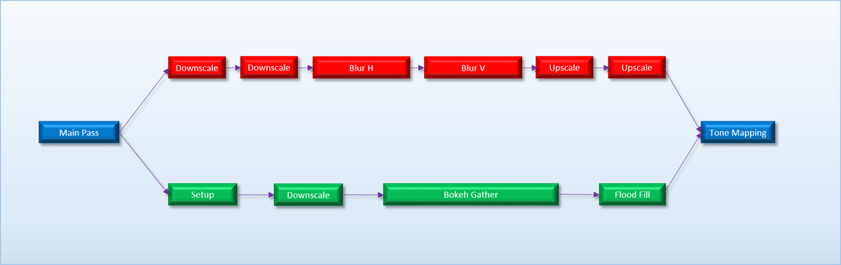
From the graph it’s clear that the bloom/DOF chains are independent while they’re executing, but they need to be synchronized at the start and end of the chains to make sure that everything works correctly. This implies that if we were to run the two chains as two separate command buffers submitted to the dual front-ends of the MJP-4000, we would need some kind of cross-queue synchronization in order to ensure correct results. Conceptually this is similar to our need for a barrier to ensure that all threads of a dispatch complete executing a dependent dispatch, except in this case we need to ensure that multiple chains have completed. If we were to use such a barrier to synchronize our post-processing chain, it would look something like this:

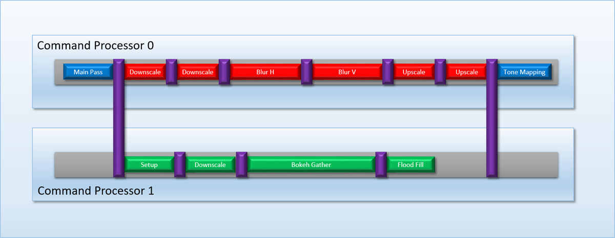
There are a few ways that this kind of cross-queue barrier could be implemented on a GPU, but the MJP-4000 takes a simple approach by re-purposing the SIGNAL_POST_SHADER and WAIT_SIGNAL instructions. Both command processors can access the same set of labels (indicated by the labels area being shared on the logical layout diagram), which gives them the basic functionality needed to wait for each other when necessary. For our bloom/DOF case we could have the DOF chain write a label when its finished, and the main command stream could wait on that label before continuing on to the tone mapping dispatch.

Next Up

In Part 4, we’ll discuss how having multiple command processors can be useful for scenarios where multiple applications are sharing the same GPU.

---

Comments:

- Dec 3, 2018

Hi, there is a niggle that for the figure of MJP-4000 work flow, at 608 cy, the threads remaining of C should be 20, not 28, and the following illustration may not be right.

---

#### []( "") - Jun 1, 2018

dude, is it based on documented source or Plato’s Cave?

---

#### [MJP](http://mynameismjp.wordpress.com/ "mpettineo@gmail.com") - Jan 3, 2019

Thank you for explaining that, Apollo. What you’re describing is exactly what I was trying to show in the diagram, but as you pointed out it’s doing a poor job of conveying that since it’s not actually showing where different commands are processed by the command processor. I’m going to re-visit that diagram, and re-work it to make it (hopefully) easier to understand.

---

#### [Apollo](http://aiellis.com "apolloiellis@gmail.com") - Jan 3, 2019

Anonymous had a good question. The second downsample has to wait for the WAITSIGNAL, since it is dependent on the first downsample writes. It can’t just run. So the graph wouldn’t look like this, unless the blue bar is the WAITSIGNAL, in which case the long dispatch would have to finish first, as he said, before another POSTSHADER signal can be used. Also in this case the diagram is not showing the POSTSHADER signal which must have been at the beginning of the dispatch since, the long dispatch ran immediately i.e at the beginning.

---

#### []( "pursue_zhao@163.com") - Dec 3, 2018

Hi MJP, I understand why now. For other guys may have the same question, I would like to post my answer here. The small blue barrier is split barrier. The first downscale is before SIGNAL_POST_SHADER and long dispatch and the second downscale is before WAIT_SIGNAL, so that the previous downscale and long dispatch can overlap and save time. But if another split barrier is added between downscale and Blur H, then its SIGNAL_POST_SHADER will wait long dispatch to complete coz long dispatch is previously-queued, so that this split barrier will be the same with a FLUSH.

---

#### []( "pursue_zhao@163.com") - Dec 3, 2018

Hi, thanks so much for your nice sharing. You mentioned in the bloom example that split barrier could only be used once if SIGNAL_POST_SHADER is limited to signaling after all previous-queued threads have completed. My question is that does the small blue barrier mean SIGNAL_POST_SHADER, and why it can be used only once ?

---

#### []( "") - May 2, 2019

Thanks for the great series here! This clause is missing its end: “There are a few ways that this kind of cross-queue barrier,”

---

#### [MJP](http://mynameismjp.wordpress.com/ "mpettineo@gmail.com") - May 2, 2019

Thank you for pointing that out!

---

#### [Breaking Down Barriers – Part 1: What’s a Barrier? – The Danger Zone](https://mynameismjp.wordpress.com/2018/03/06/breaking-down-barriers-part-1-whats-a-barrier/ "") - Mar 2, 2019

[…] 1 – What’s a Barrier? Part 2 – Synchronizing GPU Threads Part 3 – Multiple Command Processors Part 4 – GPU Preemption Part 5 – Back To The Real World Part 6 – Experimenting […]

---

#### [Breaking Down Barriers – Part 2: Synchronizing GPU Threads – The Danger Zone](https://mynameismjp.wordpress.com/2018/04/01/breaking-down-barriers-part-2-synchronizing-gpu-threads/ "") - Mar 2, 2019

[…] 1 – What’s a Barrier? Part 2 – Synchronizing GPU Threads Part 3 – Multiple Command Processors Part 4 – GPU Preemption Part 5 – Back To The Real World Part 6 – Experimenting […]