In my previous post, where I gave a quick overview of real-time subsurface scattering techniques, I mentioned that one of the potential downsides of preintegrated subsurface scattering was that it relied on sampling a precomputed lookup texture for storing the appropriate “wrapped” or “blurred” lighting response for a given lighting angle and surface curvature. Depending on the hardware you’re working with as well as the exact details of the shader program, sampling a lookup texture can be either a good or a bad thing. If you have bandwidth to spare and/or your shader is mostly bottlenecked by ALU throughput, then a lookup texture could be relatively cheap. In other scenarios it could singificantly increase the average execution time of the shader program. Either way it tends to make your life as a programmer a bit more difficult, especially when it comes to providing a suitable workflow for content creators that use your engine. In particular things get complicated if you want to allow these creators to use customizable (or arbitrary) diffusion profiles, and even more complicated if they want to be able to vary the profile spatially (imagine trying to nail the look of intricate makeup without being able to vary the scattering parameters).

If you’re skilled in the dark arts of approximating complex integrals with simpler functions, you could probably see yourself doing that for the lookup texture generated by a single diffusion kernel (and like I mentioned last time Angelo Pesce already took a stab at this for the kernel used in the original implementation of preintegrated SSS). However you would probably be less enthusiastic about doing this for a whole set of lookup textures. Instead, wouldn’t it would be much nicer if we could work with a more analytical approach that could approximate a wide range of scattering profiles without any precomputation? The rest of this post will talk about one possible way of achieving this using spherical gaussians.

Blurring A Light With an SG

Unfortunately I haven’t come up with any magical solutions for how to analytically compute the result of irradiance being convolved with a diffusion profile, even with the constraints used in the original preintegrated subsurface scattering technique (point lights, and making the assumption that the point being shaded is on the surface of a sphere). However, it turns out that we can achieve this somewhat indirectly by instead blurring the incident radiance and computing the resulting irradiance from that. It’s not the same thing conceptually, but it does produce similar results to what we’re after. The most obvious choice to do this kind of operation is probably spherical harmonics (SH): with SH we store spherical signals in the frequency domain, which makes it trivial to perform convolutions on the data (this is in fact how irradiance is traditionally computed from a set of SH coefficients representing incoming radiance). However this frequency domain representation means that we are unable to represent high-frequency components without storing and working with very large numbers of coefficients. In other words an SH approach might work well for something like an environment probe used for ambient lighting, but it can be pretty inaccurate when used for a punctual light source. To show you what I mean, here’s a comparison showing what the irradiance from a simple directional light looks like when computed analytically versus being projected onto L1 SH with 4 coefficients, and L2 SH with 9 coeffecients:

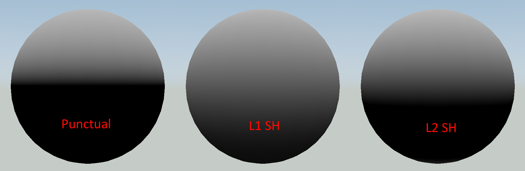
You can see quite clearly that we’re already getting a filtered, lower-frequency version of the lighting response just by going through low-order SH. This means that the SH approach can be suitable for relatively large/wide diffusion kernels, but it’s not a great fit in terms of being able to seamlessly scale from small scattering amounts to larger mean scattering distances.

As an alternative to SH, we can instead consider using our old friend the Spherical Gaussian (SG). SG’s have five properties that are of interest to us when it comes to trying to approximate the response from a filtered light source:

1. They can be oriented in any direction, which means they can be lined up perfectly with a punctual light source
2. They have an aribitrary sharpness parameter ( \( \lambda \) ) that lets them represent a range of filtering parameters, including very narrow kernels
3. An SG is trivial to normalize (when making some reasonable approximations), which ensures that we will not add or remove any energy
4. An SG convolved with a delta gives you another SG. This means we can use an SG to represent a filtering kernel, apply it to a punctional light source, and get another SG
5. We have a good approximation for computing the resulting irradiance from an SG light source

With this in mind, the approach looks fairly straightforward: first, we come up with an SG that represents the filtering kernel we will use to approximate our scattering profile. Wider kernels will have a lower sharpness parameter, while more narrow kernels will have a higher sharpness. We can then normalize the SG to ensure that it integrates to 1 over the entire sphere, which is critical for ensuring energy conservation in the filtering process. Once we have a normalized SG representing the filtering kernel, we combine it with our light source by setting the axis ( \( \mu \) ) parameter of the SG equal to the direction to the light source, and multiplying the SG’s amplitude ( \( a \) ) by the attenuated intensity of the light source. This effectively gives us an SG light source, for which we can compute the diffuse response in the usual way by using Stephen Hill’s fitted irradiance approximation and multiplying the resulting irradiance by \( \frac{albedo}{\pi} \). For scattering profiles that vary by wavelength (which is typically the case) we extend this process by coming up with a separate SG for the red, green, and blue channels and evaluating each separately. When doing this the light intensity can actually be factored out if we like, which means we can leave the SG with its normalized amplitude and multiply with the attenuated light intensity afterwards. Here’s what this all might look like in code form:

float3 diffuse = nDotL;
if(EnableSSS)
{
    // Represent the diffusion profiles as spherical gaussians
    SG redKernel = MakeNormalizedSG(lightDir, 1.0f / max(ScatterAmt.x, 0.0001f));
    SG greenKernel = MakeNormalizedSG(lightDir, 1.0f / max(ScatterAmt.y, 0.0001f));
    SG blueKernel = MakeNormalizedSG(lightDir, 1.0f / max(ScatterAmt.z, 0.0001f));

    // Compute the irradiance that would result from convolving a punctual light source
    // with the SG filtering kernels
    diffuse = float3(SGIrradianceFitted(redKernel, normal).x,
                     SGIrradianceFitted(greenKernel, normal).x,
                     SGIrradianceFitted(blueKernel, normal).x);
}

float3 lightingResponse = diffuse * LightIntensity * DiffuseAlbedo * InvPi;

For this snippet we used a very simple mapping from an arbitrary ScatterAmt parameter to an SG sharpness, where \( \lambda = \frac{1}{ScatterAmt} \). This doesn’t directly map to a diffusion kernel that’s specified in terms of distance from the shading point, but we’ll come back to that latter. First, let’s see what this looks like when we apply this algorithm for a simple directional light with various values of ScatterAmt:

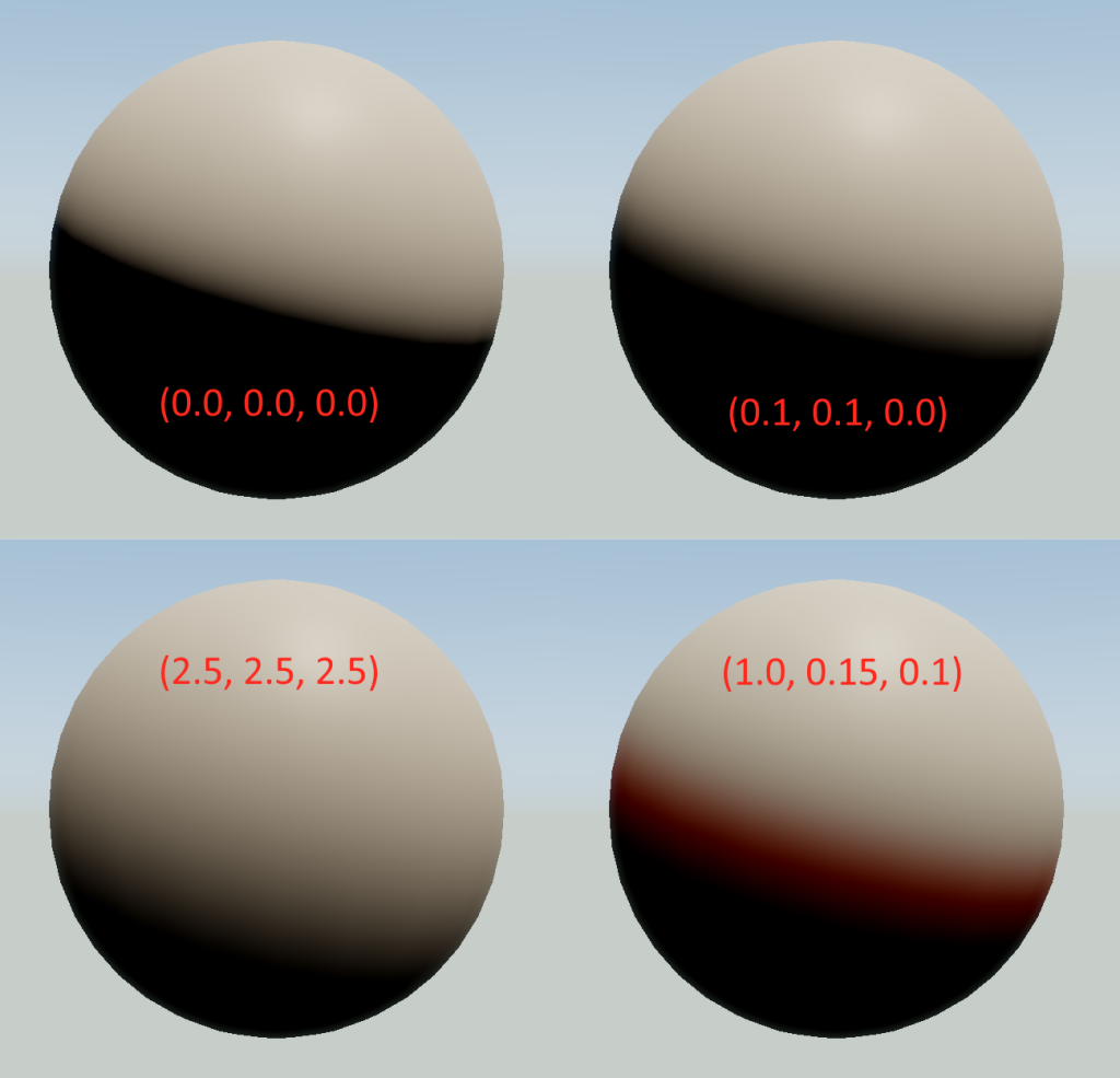
From these results, it looks like this gets us pretty close to our goal of approximating the subsurface scattering response of a point light with aribtrary scattering widths. And we’re doing all of that with pure shader math, no lookup textures required! The first image in the top-left also shows that we can scale the filtering all the way down to the “no scattering” case just fine, which is convenient.

If you wanted to optimize this further you could probably start by pulling out the portions of SGIrradianceFitted that aren’t dependent on the SG sharpness, since the normal and axis are the same for all 3 SG’s. However in practice you will probably want to combine this with the normal map prefiltering technique described in the preintegrated subsurface scattering article, since that will simulate scattering through small-scale bumps. If you do this you’ll end up with separate normal values for each channel, in which case you won’t be able to make the same optimization.

Accounting For Curvature

If you’re familiar with how preintegrated SSS works, you may have already realized a problem with our proposed technique: it’s not accounting for the curvature of the surface. If we were to just use the same set of sharpness values everywhere on an arbitrary mesh the results would not look correct, because the falloff/wrap caused by the SG would be same regardless of how flat or curved the surface is. Another way of saying this is that since our SG works purely in an angular domain, we’re effectively getting larger or smaller scattering distances across the mesh. Fortunately this problem is solvable with a bit of math. Recall that an SG has the following form:

$$ G(\mathbf{v};\mathbf{\mu},\lambda,a) = ae^{\lambda(\mathbf{\mu} \cdot \mathbf{v} - 1)} $$

or alternatively:

$$ G(\mathbf{v};\mathbf{\mu},\lambda,a) = ae^{\lambda(\cos(\theta) - 1)} $$

Since it only depends on the cosine of the angle between the sample point and the SG axis direction, the “width” of the SG is fixed in the angular domain but variable in terms of Euclidean distance if we were to vary the radius ( \( r \) ) of the sphere that it’s defined on. Therefore we need to redefine our SG in terms of Euclidean distance ( \( d \) ) between the SG center on the surface of the sphere ( \( c \) ) and the shading point ( \( s \) ), where \( \theta \) is the angle between the surface normal and SG axis (which is aligned with the light direction):

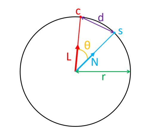
We can then use the following to get the distance between the points:

$$ d = 2r\sin(\frac{\theta}{2}) $$

If we flip that around to get the value of \( \theta \) in terms of distance, we get this:

$$ \theta = \sin^{-1}(\frac{d}{2r})2 $$

We can then plug that into the second form of the SG definition and get the following:

$$ G(d;\lambda,a,r) = ae^{\lambda(\cos(\sin^{-1}(\frac{d}{2r})2) - 1)} $$

This looks pretty gnarly, but fortunately we can simplify this by making the substitution \( \cos(2\sin^{-1}(x)) = 1 - 2x^{2} \), which gives us something much nicer once we clean it up a bit:

$$ G(d;\lambda,a,r) = ae^{\frac{-\lambda d^2}{2r^2}} $$

In case that’s too hard to read, this is the exponent part on its own:

$$ \frac{-\lambda d^2}{2r^2} $$

This is now really close to a standard 1D Gaussian form, which is pretty neat! It’s also now quite clear that the effective width of the SG will increase as the radius increases, which is not what we wanted for subsurface scattering. This is confirmed if we graph this out for a few values of \( r \):

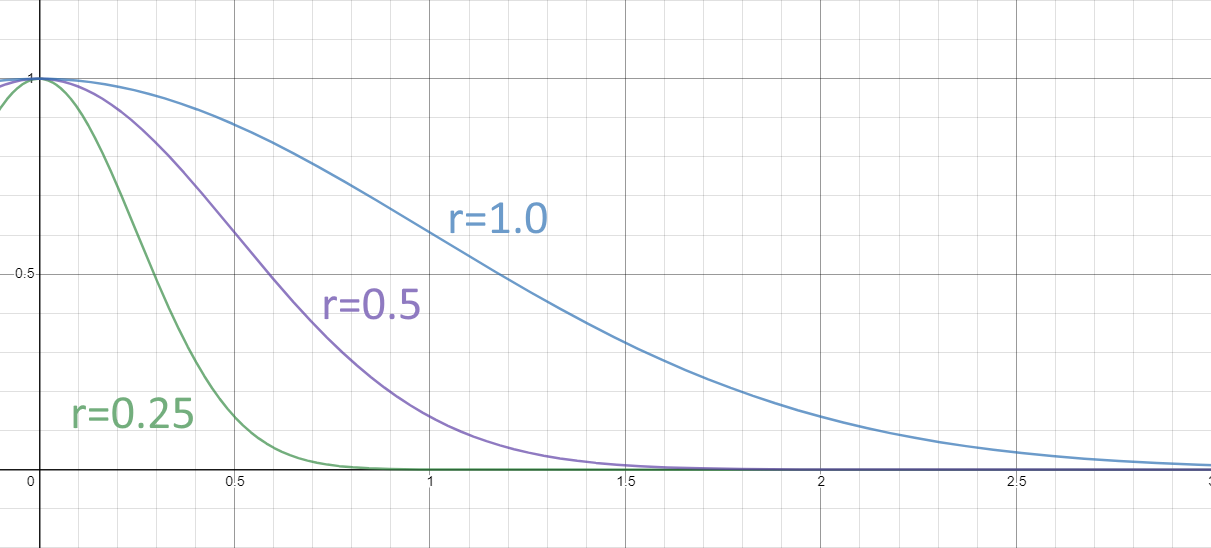
The good news is that we can fix this very easily: we just need that \( r^2 \) term to drop out, which will happen if we multiply \( \lambda \) by \( r^2 \). Doing that gives up exactly a 1D Gaussian, except with a \( \lambda \) in the numerator of the exponent instead of the usual \( \sigma \) in the denominator:

$$ G(d;\lambda,a) = ae^{\frac{-\lambda d^2}{2}} $$

This final form gives us the fixed width kernel that we’re after, as long as we can compute the effective radius from the curvature of the mesh. We can do that using pixel shader derivatives as described in the preintegrated SSS article, or we can precompute it and store it in a texture or per-vertex. This also gives another interpretation of our ScatterAmt parameter that we used earlier: it’s the \( \sigma \) parameter of a Gaussian centered around the point \( c \).

Applying To Ambient Lighting

In most real-time scenarios we’re going to be combining lighting from punctual light sources with precomputed GI stored as either spherical or hemispherical probes in 3D space. For SH probes, I already outlined a workable approach earlier in this article. Really you just need some kind of function for generating the SH coefficients for a Guassian, and then we can multiply that with the SH lighting environment to pre-filter it. Something similar to what Ravi Ramamoorthi proposed for approximating a Torrance-Sparrow NDF would probably work pretty well:

$$ \Lambda \rho \approx e^{-(\sigma l)^{2}} $$

For probes encoded as a set of SG’s, we can make use of Kei Iwasaki’s forumula for approximating the convolution of two SG’s (brought to my attention by Brian Karis’s blog post), which looks like this once implemented in HLSL:

//-------------------------------------------------------------------------------------------------
// Approximates the convolution of two SG's as another SG
//-------------------------------------------------------------------------------------------------
SG ConvolveSGs(in SG x, in SG y)
{
    SG convolvedSG;
    convolvedSG.Axis = x.Axis;
    convolvedSG.Sharpness = (x.Sharpness * y.Sharpness) / (x.Sharpness + y.Sharpness);
    convolvedSG.Amplitude = 2 * Pi * x.Amplitude * y.Amplitude / (x.Sharpness + y.Sharpness);

    return convolvedSG;
}

The approach is then similar to what we do for punctual lights: come up with the normalized SG’s for red/green/blue, convolve them with each SG in the lighting probe, and compute the resulting irradiance.

Limitations and Future Work

Compared with standard Lambertian diffuse, this approach is much more math-heavy. I have implemented and shipped this technique in two games already, so it’s definitely usable. But obviously you’ll want to be wary of the extra ALU and register pressure that it can add to a shader program.

In terms of the visual results, it mostly suffers from the same major visual drawbacks that you get with preintegrated subsurface scattering. In particular there’s no great solution for handling shadow edges, and your results may suffer if your technique for computing curvature has errors or discontinuities. It also does nothing to account for scattering through thin surfaces like the ears, so that has to be handled separately. It also shares another limitation with preintegrated SSS: it assumes punctional light sources. For area lights you would need to do something more complicated, perhaps using the LTC framework.

I also have not taken the time to come up with a more principled approach for applying the normal map prefiltering based on the ScatterAmt parameter. Currently I use a simple ad-hoc mapping from that parameter to lerp factors between the detail normal map and the base normal map, which works well enough but could certainly be improved. If anybody has thoughts on this, please let me know in the comments or on Twitter!