An Introduction To Real-Time Subsurface Scattering

A little while ago I was doing some research into the state-of-the-art for approximating subsurface scattering effects in real-time (mainly for skin rendering), and I had taken a bunch of loose notes to help me keep all of the details straight. I thought it might be useful to turn those notes into a full blog post, in case anyone else out there needs an overview of what’s commonly used to shade skin and other materials in recent games. If you’re already an expert in this area then this probably isn’t the post for you, since I’m not going to talk about anything new or novel here. But if you’re not an expert, feel free to read on!

SSS Basics

First of all, what do we mean when we say “subsurface scattering”? In reality subsurface scattering is happening even on our more “standard” materials like plastic or leather, which we typically model with a diffuse BRDF like Lambertian. This helpful image from Naty Hoffman’s 2013 talk on the physics of shading is great for understanding what’s going on:

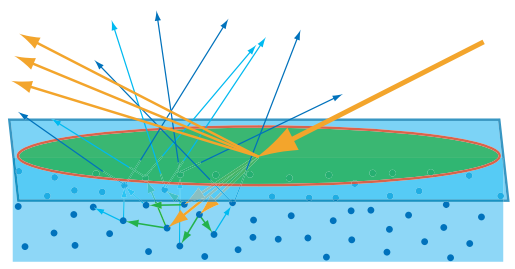
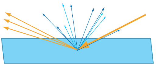
In this case you want to imagine that the green circle with the red outline is the shading area for a single pixel. The big orange arrow coming from the right is some incoming light from a particular direction, most of which reflects off the surface causing specular reflections. However some of that light also refracts into the surface, where it encounters particles within the medium. The light then scatters among the particles causing certain wavelengths to get absorbed, resulting in the light taking on the characteristic albedo color of the material. Eventually the light that isn’t completely absorbed refracts its way back out of the surface in a random direction, where it may or may not make it back to eye causing you to see it. The part that makes this easy is the fact that the scattered subsurface light all comes out within the pixel footprint. This lets us simplify things by only considering the light hitting the center of the pixel, and then estimating the amount of light that comes back out. In effect we do something like this, where we assume all of the scattered light comes out right where it initially entered the surface:

However this is not usually what we’re talking about when we mention subsurface scattering in the context of games or graphics. Usually that term is only brought up in cases where the material is particularly translucent, allowing the scattered light to bounce around even further than in more typical materials. Like in this diagram:

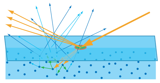
In this case the scattered light is no longer coming out within the pixel footprint, it’s coming out in areas that could possibly be covered by neighboring pixels. In other words we’ve crossed a threshold where we can no longer consider only the incoming lighting to a pixel, and we instead need to globally consider lighting from elsewhere in order to model the visible effect of light diffusing through the surface. As you can imagine this really complicates things for real-time renderers, but we’ll talk about that more in a bit.

For a moment, let’s assume we’re doing an offline render with access to ray tracing and other fancy features. How do we compute the contribution from subsurface scattering in that case? If we wanted to be really accurate, we would use volumetric path tracing techniques to compute how lighting scatters and refacts about within the medium. This probably sounds expensive (and it is!), but it’s becoming an increasingly viable option for high-end animation and VFX studios. Either way this approach lets you simulate the full path of light along with all of the various scattering events that occur under the surface, which can give you a relatively accurate result that accounts for complex geometry and non-uniform scattering parameters.

Diffusion Approximations

For games and real-time we’re obviously a lot more constrained, so instead we typically work with a more approximate diffusion-based approach. Most of the work in this area stems from Jensen’s paper published back in 2001, which was the first to introduce the concept of a Bidirectional Surface Scattering Distribution Function (BSSDF) to the graphics world. That paper spawned all kinds of interesting follow up research over the past 18 years, spanning both the worlds of offline and real-time graphics. Covering all of that is outside of the scope of this blog post, so instead I’m going distill things down to the basic approximations that we work with in games.

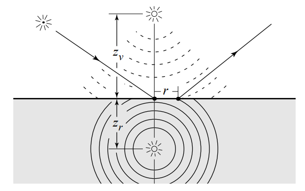
They key to Jensen’s approach is the simplifying assumption that the light distribution within a highly-scattering media tends to be isotropic. If you’re not familiar with volumetric rendering terms, what this means is that once light into the surface it’s randomly likely to end up coming out in any direction, rather than being mostly aligned to the incoming light direction or something like that. This effectively makes the scattering sort of a “blurring” function, which results in a uniform distribution of reflected lighting (note that this is basically the same assumption that we make for Lambertian diffuse). Jensen’s BSSDF was actually based on two parts: an exact method for computing the single-scattering contribtution (light that goes into the surface, hits something, then bounces right out again) and a “dipole” method that approximates the multiple-scattering contribution (light that goes into the surfaces, has multiple scattering events, and then finds its way out) by evaluating two virtual point light sources: one above the surface, and one below:

Even if you have analytical approaches for computing the scattering from an incoming point on the surface to an outgoing point, the problem is that your rendering integral just got even worse than it usually is. Evaluating an arbitrary BSSDF means computing the value of this integral:

$$ L_{o}(o, x_{o}) = \int_{A} \int_{\Omega} S(x_{i}, i; x_{o}, o) L_{i}(x_{i}, i)(i \cdot n_{i}) didA $$

That’s one mean integral to evaluate: it basically means we have to go over the entire surface of the mesh, and at every point on that surface sample every direction on the upper hemisphere and apply the scattering function \( S(x_{i}, i; x_{o}, o) \) to the incoming lighting. If we want to simplify this a bit, we can make the assumption that the scattering function is radially symmetric and really only depends on the distance between the incoming point and the outgoing point. That brings us to a somewhat less complicated integral:

$$ L_{o}(o, x_{o}) = \int_{A} R(||x_{i} - x_{o}||) \int_{\Omega} L_{i}(x_{i}, i)(i \cdot n_{i}) didA $$

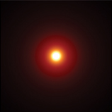
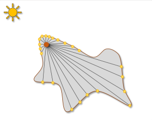
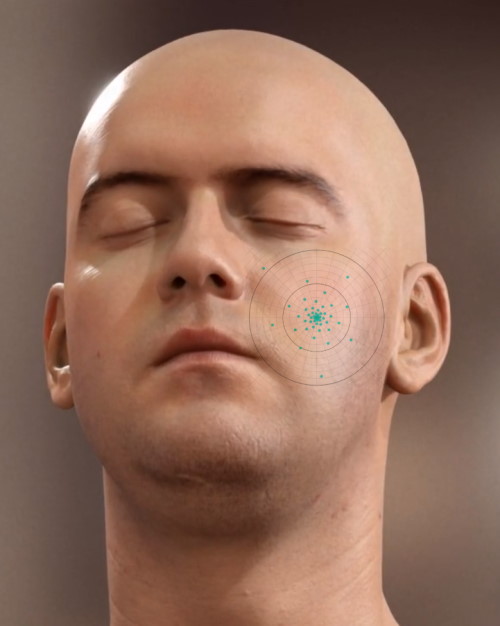
Our new integral now boils down to “for every point on the surface, compute the irradiance and then multiply that with a scattering function that takes distance as a parameter”. This is less complicated, but doesn’t fix the whole “to shade single point we need to shade every single other point on the surface” problem. However it does give us a useful framework to build on, and also a simplified mental model that we can use. The “scattering only depends on distance” assumption basically turns the scattering function into blur/filter kernel, except it’s applied to an arbitrary mesh surface instead of a 2D image. Thus you’ll often see the \( R(r) \) part referred to as as a diffusion profile (or sometimes as a diffusion kernel), which is the terminology that I’ll often use myself for the rest of this article. If you want to picture what the diffusion profile would look like for something like human skin, you’ll want to imagine that you’re in a completely dark room and could shoot an extremely narrow completely-white laser beam at your skin:

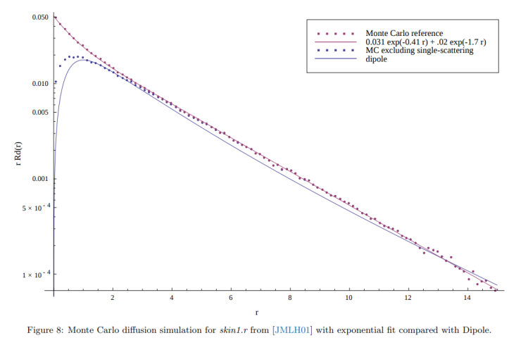
Technically speaking, you can use whatever diffusion profile you’d like here. For instance you can use a Gaussian kernel, smoothstep, cubic function, etc. However you’ll really want to work with something that’s “normalized” in the sense that it doesn’t add or remove energy (in other words, the kernel integrates to 1 for all possible configurations). There’s also no guarantee that the kernel you pick will actually be a plausible match for the scattering behavior of a real-world behavior such as skin. To do that, you have to carefully choose your diffusion profile such that it closely matches the measured (or accurately computed) response of that material. Disney did exactly this for human skin, and they created a kernel based on the sum of two exponentials that they called “normalized diffusion”. The neat thing about their model is that not only is it simple and intuitive to work with, they also showed that they could accurately fit to both the single and multi-scattering components with a single kernel:

Rendering With a Diffusion Profile

So how we do we actually render something with a BSSDF? Even with the simplifications that we get from using a radially-symmetric diffusion profile, we still have the problem that the shading for any particular surface on a mesh potentially depends on every other surface on the same mesh. In practice we can improve the situation by exploiting the fact that a well-behaved diffusion profile should always decrease in value as the distance gets larger. This lets us determine a “maximum scattering distance” where the contribution beyond that distance is below an acceptable threshold. Once we have this \( r_{max} \), we can limit our sampling to within a sphere whose radius is equal to \( r_{max} \). This definitely helps things quite a bit by letting us constrain things to local neighborhood around the shading point.

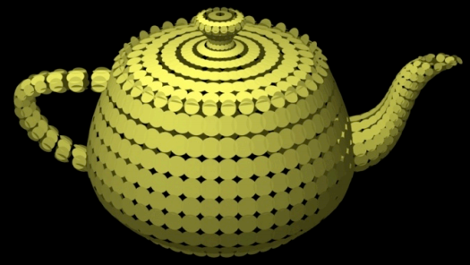
Most early uses of sub-scattering the offline world was built using around using point clouds to sample the neighboring irradiance. Point clouds are a hierachical structure that allows the illuminance to be cached at arbitrary points in the scene, typically located on the surfaces of meshes (also known as surfels):

They were popularized by Pixar, who integrated them into RenderMan in order to compute global illumination. Later on as point clouds fell out of favor and path tracing began to take over, monte carlo methods began to appear. This presentation from Solid Angle and Sony Imageworks sums up 4 such approaches, each based around the idea of distributing ray samples around the sample point in such a way that their density is proportional to the diffusion profile. The fourth method (shooting rays along within a sphere from orthogonal directions) has been used by Disney, and perhaps many others:

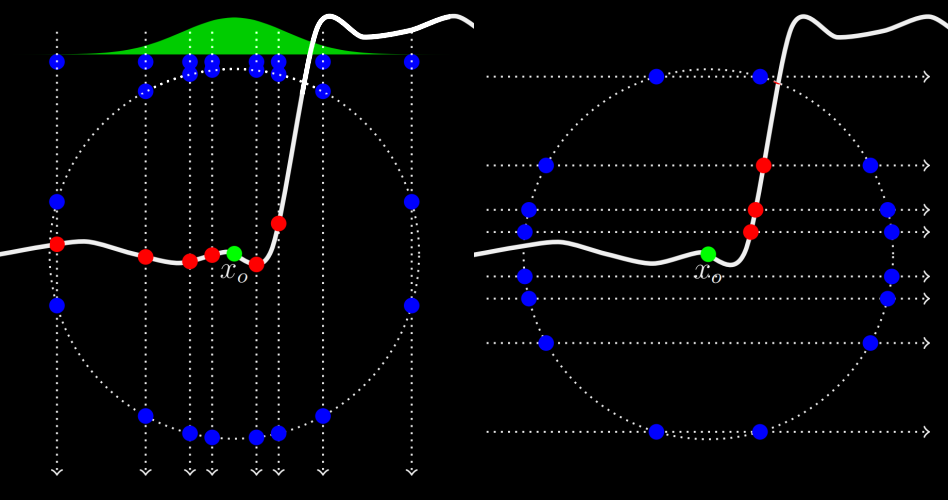
while the first method (uniformly shooting rays from a point just below the surface) has actually been used in real-time by EA SEED’s Halcyon rendering engine:

These methods can both be very effective as long as you have the resources to perform ray intersections against your scene geometry. Despite the heavy expense involved, there are still making some assumptions being made here that can be violated depending on your particular scene. In particular, each point that is hit by a ray is assumed to be “connected” to the original shading point such that it would be plausible for light to scatter all of the way there. This issue is mitigated by restricting the ray queries so that they only intersect with the same mesh being shaded, which has the added bonus of reducing the amount of surfaces that need to be considered. But even with that restriction it’s easy to imagine a scattering path that would pass right through an empty gap of air. Disney has a diagram from their course notes showing such a case:

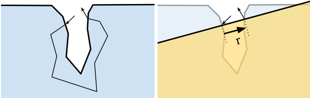
If light were to scatter all the way from the entry point to the exit point in that example, it would have to scatter all the way around the crevice which is quite a long way to go. An approach that merely consideres the distance between those points will over-estimate the scattering here, as opposed to a proper volumetric path tracer that could actually account for the gap.

Rendering Diffusion in Real-Time

So it’s great that offline renderers can just shoot a bunch of rays around in order to sample the irradiance in a local neighborhood, but until very recently it wasn’t viable to do this in real-time (and even with the latest RTX hardware you’re still only going to get a handful of rays per-pixel every frame). This meant that games generally had to fall back to even cheaper approximations in order render the skin on their hero characters. There have likely been all kinds of ad-hoc approaches used over the past 15 years or so, many of which were never presented or described anyhere. So instead of covering them all, I’m going to give a quick overview of some of the more commonly-used and referenced techniques that you’ll find out in the wild.

Texture-Space Diffusion

This approach was popularized by the incredible Human Head demo for the GTX 8800, (which you can still download on Nvidia’s site!) and described in detail in GPU Gems 3 as well as in the paper from Eurographics 2007. The technique actually comes from the film world: it was first used and documented as part of the production of The Matrix Reloaded way back in 2003. Eugene d’Eon and David Luebke were able to show that it could also work in real-time on (at the time) high-end GPUs, and in the process they were able to create some visuals that are still impressive today. It’s called “texture-space” because all of the scattering/diffusion simulation happens in 2D using the UV parameterization of the head/face mesh, as opposed doing it per-pixel in screen-space. A simplified explanation of the algorithm would go something like this:

• Draw the mesh using a special vertex shader that sets output.position = float4(uv * 2.0f - 1.0f, 0.0f, 1.0f); and a pixel shader that outputs the irradiance from dynamic + baked lighting, effectively computing an irradiance map in texture-space
• Blur the irradiance map with bunch of Gaussian kernels, with a horizontal + vertical pass for each kernel (they approximate skin’s diffusion profile as a sum of separable gaussians)
• Draw the mesh for real using the camera’s projection matrix, then in the pixel shader sample the convolved irradiance maps and apply the diffuse albedo map to get the diffuse reflectance with subsurface scattering.

Obviously their results speak for themselves in terms of quality, so I don’t think that would be the main issue preventing adoption. It’s also fairly flexible in that in can handle many different diffusion profiles, provided that they can be represented as a sum of Gaussians. However there are definitely some issues that become obvious pretty quickly if you think about it:

• Shading in texture-space can be difficult to tune in terms of performance and memory usage. Shading in a pixel shader means that your shader invocations naturally drop as the mesh gets further from the camera, since the mesh will occupy less are a in screen-space. However with texture-space shading you will shade however many texels are in your off-screen irradiance buffer, so you need to manually reduce the buffer size based on the distance to the character. Ideally you would want to match the mip level that will be sampled by the mesh during the primary rasterization path, but there could potentially be a wide range of mip levels used depending on the complexity of the mesh and the camera’s current position. Budgeting enough memory for the irradiance buffer can also be difficult if you have many characters on-screen at once, especially if sudden camera cuts will cause a particular character to suddenly be in a close-up. And don’t forget that you lose z-buffer occlusion and backface culling when shading in texture-space, which means that the naive approach could potentially result in shading a lot of surfaces that never contribute to the final image!

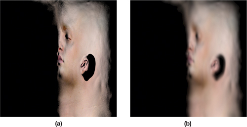
• In general, texture-space diffusion makes sense because of the assumption that the local neighborhood of a surface will also be local in the UV mapping. Most of the time this is correct, but any UV seams will break this assumption and cause ugly artifacts without somekind of workaround. It also fails for thin surfaces like the ear, since both sides of the ear are probably not going to be close in UV space. The demo accounts for the forward-scattering through thin surfaces by rendering a translucent shadow map that records the UV coordinate of the closest depth for each texel, which is then used by the surface on the “other side” to sample the blurred irradiance map at the point where the light ray hit the mesh.

• Typically the UV mapping of something like a face will have lots of stretching and warping, which would also result in a warping of the diffusion profile itself once the results are mapped back to world space: The Nvidia demo works around this by rendering out a “stretch map” in texture-space that contains the U/V distortion factors, which can then be used to modify the diffusion profile weights. You can pre-compute this map, but it will be incorrect in the case of extreme deformations from skinning or blend shapes. In those cases computing the stretch map on the fly would produce better results.

• The demo used 6 large Gaussian blur kernels to approximate the skin diffusion profile, which is a lot of passes! There was a Shader X7 article where John Hable described a simplified version were all 6 passes were collapsed down to a single 12-tap pass that could be done in the pixel shader when sampling the irradiance map. Unfortunately there’s no online version of that article, but he describes it a bit in this presentation from SIGGRAPH 2010.

• Specular shading is done in the pixel shader during the primary rasterization pass, which means that light sources need to be effectively sampled twice. An alternative would be to compute the specular in texture-space, and output it to a separate render target that’s sampled during the rasterization pass.

• The additional complexity of integrating a special-case texture-space rendering path for characters could potentially add a high maintenence cost, and may not play nice with other passes that are typically done in screen or camera space (for instance, binning lights in a frustum-aligned grid).

I’m not sure if any game actually shipped with this approach (or something) similar at runtime. Uncharted 2 used the approach described by John Hable for offline-rendered cinematics, but at runtime they fell back to something much simpler and cheaper. There was an old ATI demo that did texture-space diffusion 3 years before d’Eon and Luebke published their work at Nvidia, but what they describe sounds much less sophisticated. Overall the lack of adoption isn’t terribly surprising given the large list of potential headaches.

Update 10/7/2019: Vicki Ferguson was kind enough to point out that FaceBreaker shipped with texture-space diffusion way back in 2008! Angelo Pesce then explained how this tech made its way into the Fight Night series, where it eventually evolved into pre-integrated subsurface scattering! See Vicki’s GDC presentation and Angelo’s “director’s cut” slide deck for more info on the tech used for Fight Night Champion.

Screen-Space Subsurface Scattering (SSSS)

Once it became clear that texture-space diffusion would be both difficult and expensive to use in a real-time game scenario, a few people started looking into cheaper options that make use of lighting data stored in screen-space buffers. The idea was popularlized by the work of Jorge Jimenez, thanks to a very popular article that was published in the first edition of GPU Pro. Morten Mikkelsen (of MikkT fame) also did some early work in this area, and Jorge continued to publish additions and improvements in the following years. The state-of-the-art is probably best represented by Evgenii Golubev’s presentation from SIGGRAPH 2018, where he explained how Unity adopted Disney’s Normalized Diffusion profile for real-time use.

At a high level you’re making a similar bet that you make with texture-space diffusion: you’re hoping that 3D locality of a sample point’s neigboring surfaces is preserved when it’s rasterized and projected into 2D. When this is the case (and it often is) then you merely have to do a few texture fetches from neighboring texels in order to convolve the lighting with your diffusion profile. This is quite a bit more appealing than shading a surface in unwrapped UV space (especially on 2009-era hardware and APIs), since you can borrow from typical deferred approaches in order to output per-pixel irradiance to a secondary render target. This spares you from having to figure out the appropriate shading rate to use for the surface, and also prevents you from inadvertantly shading pixels that end up being occluded by other opaque surfaces.

With those advantages it’s not surprising that many engines ended up adopting SSSSS and using it in shipping games. But of course it’s not all roses, either. Let’s go through some of the issues that you can run into:

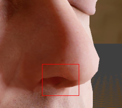
• Since you’re working in screen-space, you can only gather irradiance from surfaces that end up getting rasterized. This means that anytime you have some complex occlusion going on (for instance when the nose occludes parts of the cheek) you’re going to end up with missing information. It’s really the same problem that you can get with SSAO or SSR.

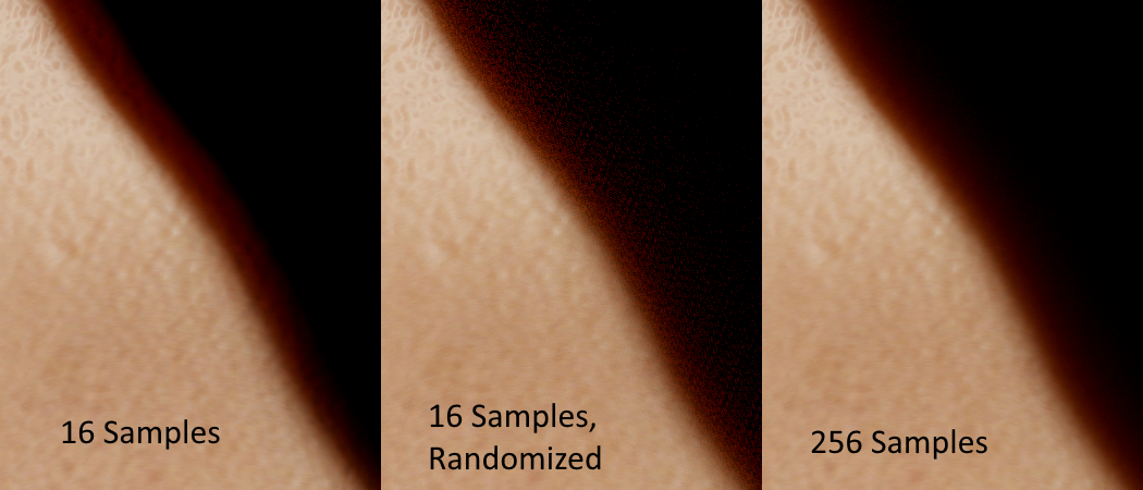
• Generally you’re going to be limited in the number of samples that you can gather, which is going to lead to undersampling. This will manifest as banding or “blobiness” if re-using the same sample pattern across all pixels, or as noise if using stochastic sampling. The latter can be mitigated with denoising and/or TAA.

• Doing things in screen-space necessitates doing the rendering in multiple passes, meaning you can’t just completely shade the surface within a single pixel shader. This is unfortunate if everything else is forward rendered, especially since it means you may need to eat the memory of a few extra render targets that are only used for a subset of materials.

• If you only want to run the SSSSS pass on pixels that require it, then you need some kind of system for tagging those pixels and selectively running the shader. Jorge’s original implementation used stencil, but I’ve never met a graphics programmer that enjoyed using stencil buffers. As an alternative you can branch on a per-pixel value, or run a pass to generate a list of screen-space tiles.

• Similar to texture-space diffusion, you can’t really account for light that transmits through thin surfaces like the ear. There might be some cases where both sides of the surface are visible to the camera, but in general you can’t rely on that. Instead of you have account for that separately, using shadow map depth buffers and/or pre-computed thickness maps. I would suggest reading through the slides from this presentation by Jorge for some ideas.

Pre-integrated Subsurface Scattering (SSSS)

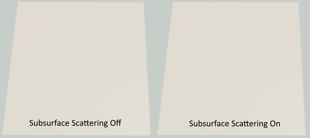
The previous two techniques were all about turning diffusion into a gathering problem: one gathered local irradiance in texture-space, the other in screen-space. There’s some key differences that we already covered, but fundamentally they’re trying to do the same thing, just in different domains. Pre-integrated subsurface scattering takes a complelely different approach: it makes no attempt at all to look at the lighting in the local neighorhood. Instead, it tries pre-compute the scattered results, and use the correct result based on a few properties of the point being shaded. The key insight that Eric Penner presented was that subsurface scattering isn’t actually visible in cases where the surface is totally flat and the incoming lighting is uniform across the surface. It’s like opening up an image in photoshop where every pixel has the same color and then running a Gaussian blur filter on it: you won’t see any difference, since you’re just blurring the same color with itself. We can confirm this pretty easily by running ray-traced diffusion on a plane lit by a single direction light, and comparing it with the result you get without subsurface scattering:

Totally worth all of the cost all of those rays, am I right? If we know that you don’t see subsurface scattering when the the light is uniform and the surface is flat, then we can deduce that the scattering will be visible whenever those two things aren’t true. A quick test with our ray-tracer can confirm our hypothesis. Let’s first try a sphere to see what happens when the surface isn’t flat:

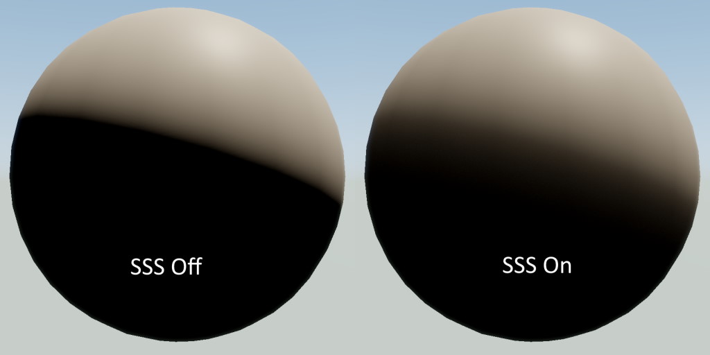
In this case the difference is huge! Now let’s look at an example where the lighting changes very quickly due to a shadow being cast by another mesh:

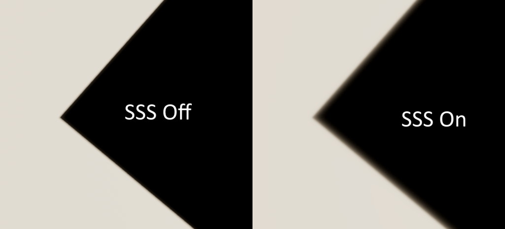
This time we see the lighting diffusing its way over into the shadowed pixels, which is very noticeable. Really these are both two sides of the same coin: the incident irradiance is varying across the surface, in one case due to the changing surface normal and the other due to changes in light visibility.

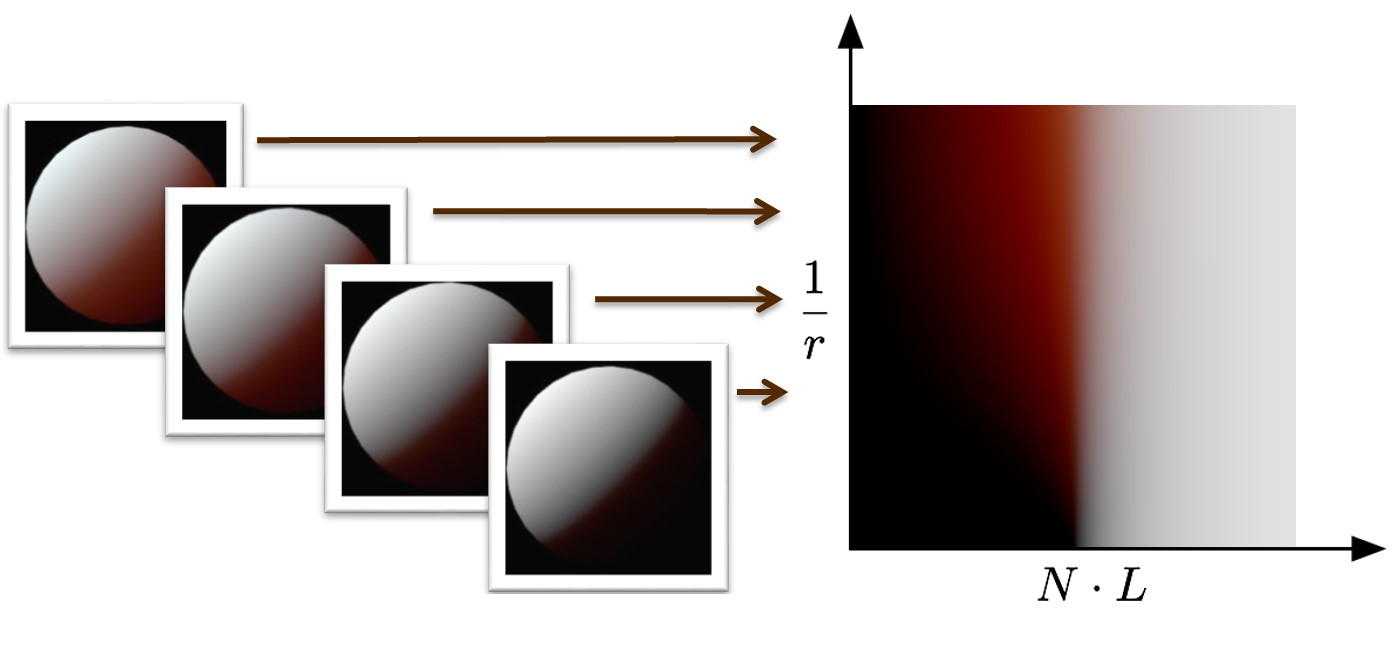
Eric decided to tackle these two things separately in his presentation, so let’s do the same and start with the case where scattering is visible on a non-flat surface. When a surface is curved, the incident irradiance will decrease on that surface as \( N \cdot L \) decreases which is what gives you that characteristic diffuse falloff. However with subsurface scattering effectively “blurring” the incident irradiance, the appearance of that falloff will change. This is particulaly noticeable at the point where \( N \cdot L = 0 \), since in the example with SSS enabled the lighting actually “wraps” right over that line where it would normally terminate. In fact, an old trick for approximating subsurface scattering is to deliberately modify the \( N \cdot L \) part of the lighting calculations in order to produce a result that resembles what you get from SSS. Eric took this idea and made it more principled by actually precomputing what the falloff would be if you used the diffusion profile predicted by the dipole model. The way you do this is to take a circle, and then compute the resulting falloff for every point on that circle by integrating the incident irradiance multiplied with the diffusion profile:

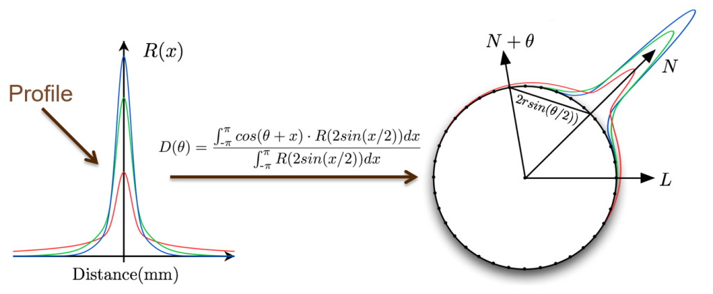
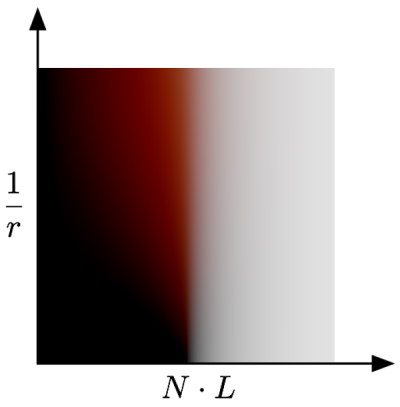
This ends up being a kind of convolution on the surface of a circle, which fits well with our mental model of SSS being a filtering operation. Doing this for the whole circle would give you a result for every value of \( \theta \) in the range \( [ -\pi, \pi ] \), but the result is symmetrical so we can discard half of the results and just keep everything from \( [ 0, \pi ] \). We can also switch from parameterizing on \( \theta \) to parameterizing on \( cos(\theta) \) in the range \( [ -1, 1 ] \), which gives us a nice 1D lookup table that we can index into using any result of \( N \cdot L \). Visualizing that would give us something like this:

This is immediatly usable for rendering, but with a major catch: it only works for a sphere with a particular radius and diffusion profile. However we can easily extend this into a 2D lookup table by computing the resulting falloff for a range of radii:

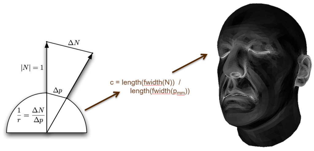
At this point you might be thinking “this is neat for spheres, but how do we use this for an arbitrary mesh?”, which is a valid question. To use this new 2D lookup texture, we need to basically take every shaded point on the mesh and map it to a sphere of a particular radius based on the local curvature of that point. Once again this was not a new idea at the time Eric presented: there was previous work from Konstantin Kolchin and Hiroyuki Kubo that had made the obvervation that subsurface scattering appearance was tied to surface curvature. Really the idea is pretty simple: figure out the local curvature, map that to a sphere radius, and then use that to choose the appropriate row of the preintegrated falloff lookup texture. Penner proposed a way to do this on-the-fly in a pixel shader by making use of pixel quad derivatives and little bit of geometry:

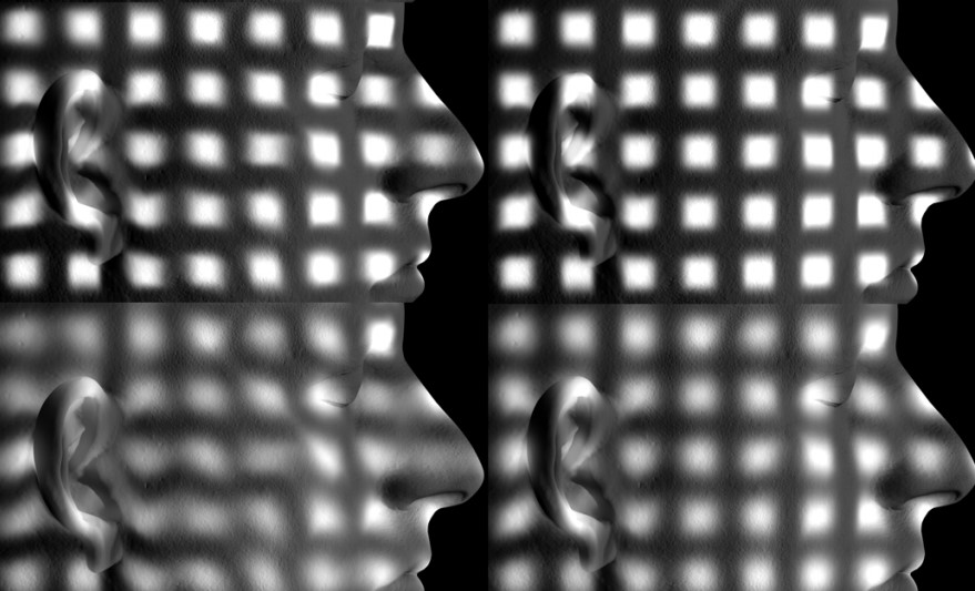
Very cool! This works…at least for curvature that’s broad enough to be captured accurately by the pixel quad derivatives. A normal map used for a human face will typically have many small bumps and other high-frequency details, and we need special-case handling if want them to look correct. Penner took inspiration from a paper called Rapid Acquisition of Specular and Diffuse Normal Maps from Polarized Spherical Gradient Illumination, which effectively pre-filtered subsurface scattering into the normal maps it produced by generating separate normals for red, green, and blue channels:

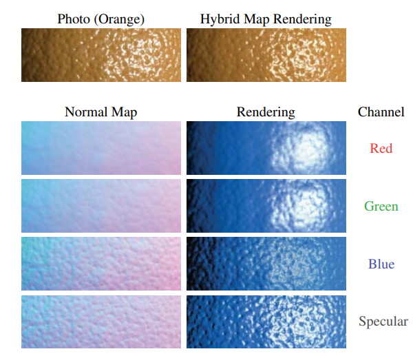
You can think of it this way: by “flattening” the red channel more than the blue, the red light will appear to have more diffusion through the bumps. Instead of requiring three seperate normal maps, Eric instead proposed sampling from the same normal map 3 different times with 3 separate mip bias amounts (one for each color channel). This provides a similar result without requiring seperate per-channel normal maps, and also allows you to use the same normal map for specular shading.

With large and small-scale curvature accounted for, we now have to look at how we handle cases where the incoming lighting changes due to shadowing. Penner’s approach to solving this was to try to determine a pixel’s location relative to the start and end of the shadow penumbra, and us that location to index into another lookup texture containing pre-integrated scattering values for various penumbra widths:

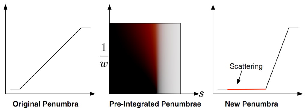
One catch here is that you can’t just apply this penumbra scattering in only the penumbra region: the scattering should actually extend past the point where the penumbra reaches zero. This is why the above diagram remaps the penumbra into a smaller area (essentially narrowing it), and then has the red “scattering” zone where the penumbra reaches zero.

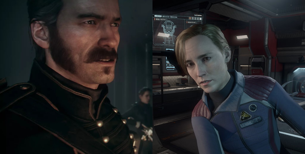
With all of these cases handled Penner was able to achieve some great results! This is quite remarkable, since this can all be achieved within the local context of a single pixel shader. This makes it possible to implement as a special shader permutation within a forward renderer, without having to implement additional passes to handle diffusion in texture-space or screen-space. It was for this reason that we shipped with a variant of this technique in both The Order: 1886 and Lone Echo, both of which use a forward renderer:

While the results speak for themselves, we also encountered many challenges and limitations:

Please note that I’ve spent a lot of time working with pre-integrated SSS, since it’s what we’ve always used in our engine at RAD. So it’s likely that the length of this list is a reflection of that, and that the list of downsides for the other techniques would be longer if I had more hands-on experience with them.

• In practice, we found that using quad derivatives to compute the surface curvature produced poor results in some cases. Eric mentioned this in his presentation, but quad derivatives will always produce values that are constant cross a triangle (you can actually see this quite clearly in the image that I used earlier). This means that you get a discontinuity at every triangle edge, which can manifest as a disconinuity in your diffuse shading. It’s not always noticeable, but when it is it can be quite distracting. You can actually see some of these artifacts in the images from the powerpoint slides if you look closely: These artifacts could also sometimes become even more noticeable due to vertex deformations from skinning and/or blend shapes, which was a real problem for using this on human faces. For these reasons we almost always ended up using pre-calculated curvature maps instead of trying to compute the curvature on the fly. The results become incorrect under deformation or scaling, which is unfortunate. But we found it was more desirable to have smoother and more consistent results.

• The original presentation and GPU Pro 2 article only explains how to handle lighting from point light sources. This means you’re on your own when it comes to figuring it out how to integrate it with baked lighting from lightmaps or probes, with the exception of the normal map prefiltering which works for any light source. While working on The Order I came up with a solution that worked with our (at the time) L2 spherical harmonics probes, which we explained in the course notes from our SIGGRAPH 2013 presentation. There’s also things you can do with spherical gaussians, but I’ll go into more detail about that in a follow-up post. Either way screen-space and texture-space diffusion can handle this naturally without any special considerations.

• I haven’t thought about it too much, but as of right now I have no idea how you would integrate this technique with area lights using LTC’s or similar approaches.

• Relying on a lookup texture can potentially be undesirable from a performance and shader architecture point of view. On some hardware it can definitely be preferable to do a pile of math instead of a texture sample, but you can’t do that without fitting some kind of approximate curve to the pre-computed data. Angelo Pesce took a stab at doing this after the original SIGGRAPH presentation, and he shared his results in two blog posts.

• For any particular diffusion profile, the technique requires two 2D lookup textures (or two fitted curves). This makes it difficult to support arbitrary diffusion profiles, since it would require generating custom lookup textures (or curves) for each material with a unique profile. Supporting a spatially-varying profile is even more challenging, since you would now need to interpolate between multiple textures or curves. Storing them as a bunch of 2D tables within the slices of a 3D texture is a doable (but expensive) option for achieving this. In a follow-up post I’ll talk a bit about a technique I came up with that side-steps this particular issue.

• I’ve found the proposed solution for handling scattering within shadow penumbras to be difficult to work with in practice. In particular I’m not sure that there’s a reliable way to estimate the penumbra width. Quad derivatives tend to produce poor results due to the reasons mentioned earlier, and the surface slope isn’t enough without also knowing the size of the “penumbra” that’s generated by filtering. And of course there’s not even a guarantee that you’ll be using a box filter for your shadow filtering, since it’s totally reasonable to use a Gaussian or some other kernel. Techniques that rely on dithering and TAA resolve would also completly break this, as would any techniques that approximate translucent shadows from things like hair (we’ve always done some tricks with VSM/MSM to approximate translucent shadows from hair). Even if you are able to perfectly reconstruct the penumbra size and the pixel’s position within it, you’re not even guaranteed that the penumbra will be wide enough to give you the appropriate scattering falloff. The Order was filled with close-up shots of faces with tight, detailed shadows.

• Using pre-integrated diffusion based on curvature and \( N \cdot L \) means you’re making the assumption that the visibility to the light source is constant over the sphere. This is obviously not always true when you have shadows. In fact it’s not even true for the simple case of a sphere, since a sphere will always shadow itself where \( N \cdot L \) is less than 0! Wide shadow penumbras and the penumbra diffusion approximation can hide the issues, but they’re always there. The worst case is something with relatively high curvature (or scattering distance) but a very tight penumbra. Here’s an example: What’s really ugly about this particular scenario is that the artifacts reveal the underlying topology of the mesh. We normally shade a virtual curved surface formed by smoothly interpolating vertex normals, but the depth rasterized into a shadow map follows the exact surface formed by the triangles. We often ran into this artifact on our faces when using tight shadows, particularly if the curvature map had too high of a value.

• The proposed technique for handling small-scale scattering through bumps in the normal map is implicitly making some assumptions about the size of the features in said normal map. In general it works best when the normal map only contains small pore-level details, but in games it’s common to also bake larger-scale curvature into the normal map when transfering from a high-resolution sculpt to an in-game mesh. You may find that you get better results by separating these two things as “base” and “detail” normal maps, and only applying the pre-filtering to your detail map. We switched to doing this for Lone Echo, and while it’s more expensive we prefer the higher-quality results. It’s also possible to use a smaller tiling detail map instead for noisy pore-level details, which can certainly save some memory.

• Like the other techniques mentioned in this article, you’ll need additional tech if you want to handle diffusion through thin surfaces like ears. Our artists would sometimes try to fake this with pre-integrated SSS by making the curvature abnormally high, but this has the effect of flattening out the front-facing lighting (since it essentialy assumes the light has diffused everywhere on the sphere).

Conclusion

Hopefully this post has helped give you a basic understanding of how subsurface scattering works, and how it can be approximated in real-time graphics. Perhaps it will also give you enough information to make a preliminary decision about which technique to use for your own real-time engine. If you were to ask me right now to choose between the 3 techniques that I discussed, I would probably go with the screen-space option. In general it seems to have the least corner cases to handle, and most closely resembles a ray-tracing approach. But that could also be a bit of “the grass is always greener” syndrome on my part. I also fully expect a few games to start using ray-traced SSS on high-end hardware at some point in the near future, since you can use that for high-quality results while keeping a screen-space path as a fallback for weaker hardware. You could also do a hybrid approach similar to what DICE did for reflections in Battlefield V, where you use screen-space for most pixels and only use ray-tracing in areas the necessary data isn’t present on the screen.

Please feel free to reach out in the comments or on Twitter if you have questions, or if you spot something incorrect that I should fix!