Signal Processing Primer
For a theoretical understanding of aliasing and anti-aliasing, we can turn to the fields of signal processing[1] and sampling theory[2]. This article will explain some of the basics of these two related field in my own words, taking a more theoretical point of view. In the following article the concepts covered here will be used to analyze common aspects of real-time graphics, so that we can describe them in terms of signal processing. If you’d like some further reading, I’d recommend consulting chapter 7 of Physically Based Rendering[3] (available as a free download), chapter 5 of Real-Time Rendering, 3rd Edition[4] or Principles of Digital Image Synthesis[5] (which is also freely available for download)
As always, I’m more interested in the material being correct than I am in sounding like I’m smart. So if you see anything that you feel is incorrect or have any additional insights to share, please let me know in the comments!
Sampling Theory
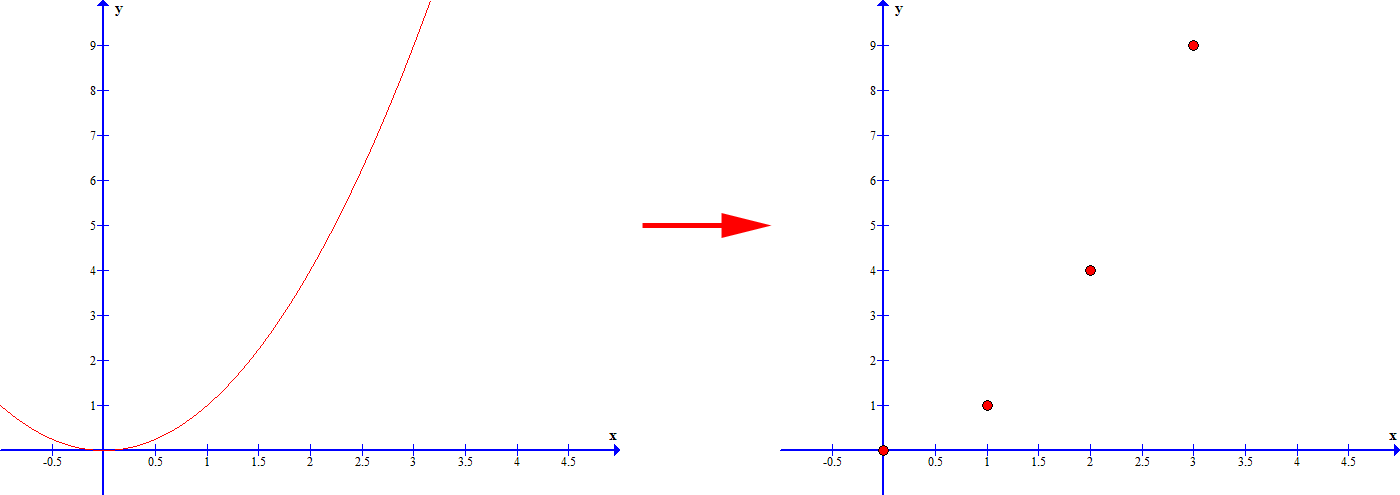
Sampling theory deals with the process of taking some continuous signal that varies with one or parameters, and sampling the signal at discrete values of those parameters. If you’re not familiar with signals and signal processing, you can think of a signal as some continuous function of any dimension that varies along its domain. To sample it, we then calculate that function’s value at certain points along the curve. Usually the points at which we sample are evenly-spaced apart, which we call uniform sampling. So for instance if we had a 1D signal defined as f(x) = x^2, and we might sample it at x =0, x = 1, x = 2 x = 3, and so on. This would give us our set of discrete samples, which in this case would be 0, 1, 4, 9, and continuing on in that fashion. Here’s an image showing our continuous function of f(x) = x^2, and the result of discretely sampling that function at integer values of x:
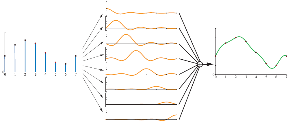
Working with discrete samples has a lot of advantages. For instance, it allows us to store a representation of an arbitrary signal in memory by simply storing the sampled values in an array. It also allows us to perform operations on a signal by repeatedly applying the same operation in a loop for all sample points. But what happens when we need the value of s signal at a location that we didn’t sample at? In such cases, we can use a process known as reconstruction to derive an approximation of the original continuous function. With this approximation we can then discretely sample its values at a new set of sample points, which is referred to as resampling. You may also see this referred to as interpolation in cases where local discrete values are used to compute an “in between” value.
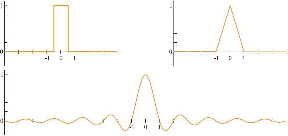
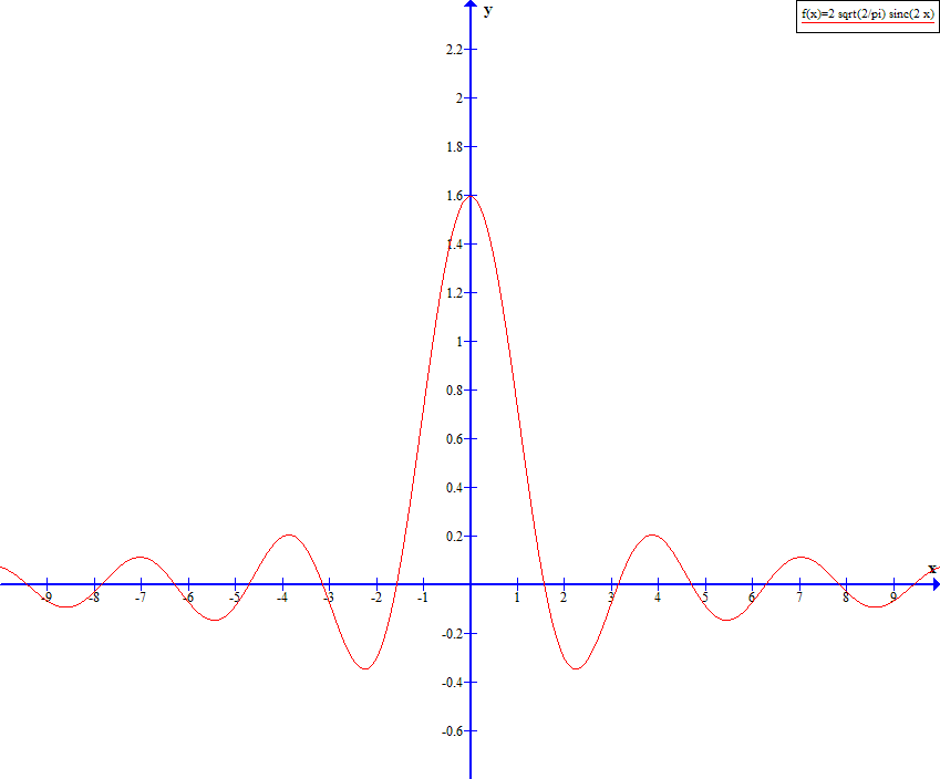
The actual process of reconstruction involves applying some sort of reconstruction filter to a set of discrete samples. Typically this filter is some function that is symmetrical about x=0, often with non-zero values only in a small region surrounding x=0. The following image contains a few functions commonly used as reconstruction filters:
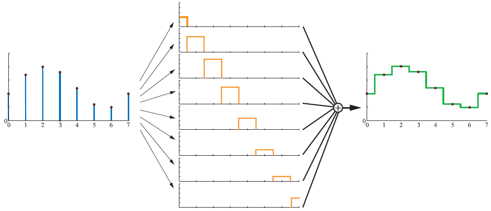
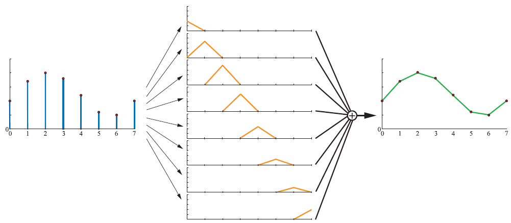
The filter is applied using a process known as convolution. In the case of discrete sample points, a convolution implies multiplying the sample values with an instance of the filter function translated such that it is centered about the same point, and then summing the result from all sample points. If you’re having trouble understand what this means, take a look at the following three images which show the result of convolution with three common reconstruction filters:
If you’ve ever written a full-screen Gaussian blur shader, then you’ve used convolution. Think about how you would write such a shader: you loop over nearby pixel values (sample points) in a texture, multiply each value by the Gaussian function evaluated using the distance from your output pixel, and sum the results. Evaluating a function using the distance to the sample point is equivalent to translating the filter function to the location of the sample point, although you may not have thought of it this way.
Of the common reconstruction filters, the sinc filter is particularly interesting. This is because it is theoretically possible to use it to exactly reconstruct the original continuous signal, provided that the signal was adequately sampled. This is known as ideal reconstruction. To define what “adequately sampled” means for a continuous signal, we must now discuss aliasing.
Key Takeaway Points:
- Continuous signals(functions) can be sampled at discrete sample points
- An approximation of the original continuous signal can be reconstructed by applying a filter to the discrete sample values
Frequency and Aliasing
Signals are often described in terms of their frequency, which in rough terms describes how quickly a signal changes over their domain. In reality a signal is not composed of just one frequency, but can have an entire spectrum of frequencies. Mathematically a signal can be converted from its original representation (often referred to as the time domain or spatial domain, depending on the context) to its spectrum of frequencies (known as the frequency domain) using the Fourier transform. Once in the frequency domain, it can be determined if there is some maximum frequency where all frequencies above that have an intensity of zero. If such a maximum frequency exists, the signal is said to be bandlimited, which means we can determine the bandwidth of that signal. Depending on the context, the term “bandwidth” can be either the passband bandwidth or the baseband bandwidth. The passband bandwidth is equal to the maximum frequency minus the minimum frequency, while the baseband bandwidth simply refers to the refers to the maximum frequency. With sampling theory we are primarily concerned with the baseband bandwidth, because it is used to determine the Nyquist rate of the signal. The Nyquist rate is minimum rate at which the signal should be sampled in order to prevent aliasing from occurring, and it is equal to 2 times the baseband bandwidth. The term “aliasing” refers the fact that a signal can become indistinguishable from a lower-frequency signal when undersampled. The following image demonstrates this phenomenon with two sine waves of different frequencies, where the samples would be the same for either signal:
In practice, aliasing that occurs due to undersampling will result in errors in the reconstructed signal. So in other words, the signal you end up with will be different than the one you were originally sampling. For signals that are not bandlimited, there is no maximum frequency and thus there is no sampling rate that won’t result in aliasing after reconstruction.
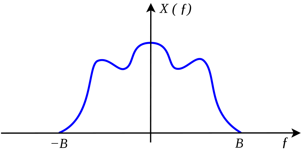
To better understand how and why aliasing occurs, it can be helpful to look at things in the frequency domain. Let’s start with the plot of the frequency spectrum for an arbitrary signal:
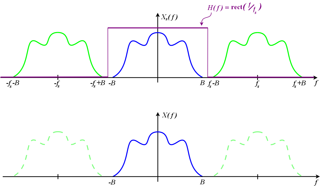
As we can see from the plot, there is a maximum frequency located at point “B”, meaning that the signal is bandlimited and has a bandwidth equal to B. When this signal is discretely sampled, an infinite number of “copies” of the signal will appear alongside the original at various points. Here’s an image illustrating how it looks:
The location of the signal duplicates is determined by the sampling rate, which is marked as “fs” in the plot. Since these duplicates are present, we must use a filter (the reconstruction filter) to remove these duplicates and leave us with only the frequency spectrum that was within the original signal’s bandwidth (referred to as the baseband frequencies). The obvious solution is to use a box function in the frequency domain, since a box function implies multiplying a certain range of values by 1 and all other values by 0. So if we were to use a box function with a width of B, we would remove the duplicates while leaving the original signal intact. The following diagram shows how this might work:
What’s important to keep in mind is that we typically need to apply our reconstruction filter in the spatial domain, and not in the frequency domain. This means that we need to use the spatial domain equivalent of a box function in frequency space, and it turns out that this is the previously-mentioned sinc function. By now it should make sense why the sinc function is called the ideal reconstruction filter, since it has the ability to leave certain frequency ranges untouched while completely filtering out other frequencies. For this same reason it is also common to refer to the frequency domain box function as the ideal low-pass filter.
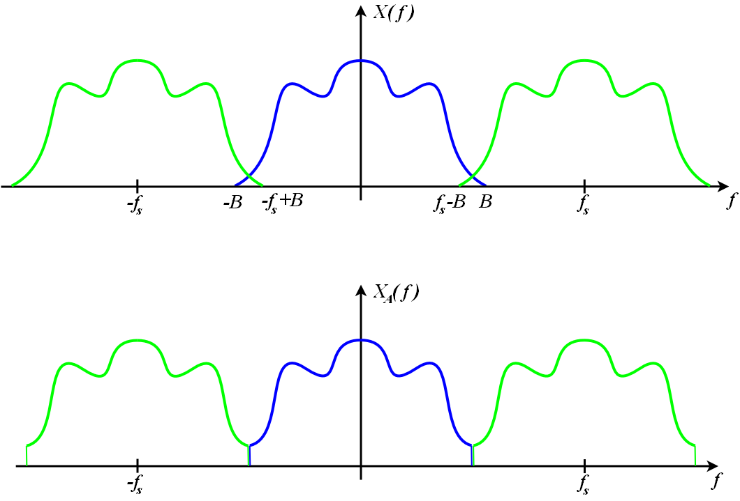
Now let’s look at what happens when we don’t sample the signal at an adequate rate. As we saw earlier, the duplicates of a signal will appear at multiples of the sampling frequency. So the higher our sampling rate the further apart they will be, while the lower our sampling rate the closer they will be. Earlier we learned that the critical sampling rate for a signal is 2B, so let’s look at the plot of a signal that’s been sampled at a rate lower than 2B:
Once we dip below the Nyquist rate of the signal, the duplicates begin to overlap in the frequency domain. After this happens it is no longer possible to isolate the original copy of the signal with a sinc filter, and thus we end up with aliasing. The bottom plot in the above image demonstrates what an alias of the original signal would look like. Since its frequency response is identical to that of the original signal, it is completely indistinguishable.
Key Takeaway Points:
- Signals can be decomposed into a spectrum of frequencies, with the spectrum being tied to the rate of change of the signal
- Signals with a maximum frequency are bandlimited
- A signal’s Nyqust rate is equal to two times its maximum frequency, and this is the minimum sampling rate required to perfectly reconstruct a signal without aliasing
- Signal reconstruction can be viewed as the process of removing “replicas” of a signal’s spectrum in the frequency domain
Reconstruction Filter Design
Aliasing that results from undersampling is referred to as prealiasing, since it occurs before reconstruction takes place. However it is also possible for artifacts to occur due to the reconstruction process itself. For instance, imagine if we used a box function that was too wide when applying a reconstruction filter. The result would look like this:
With such a reconstruction we would still end up with artifacts in the reconstructed signal, even though it was adequately sampled.
As we’ve demonstrated, using the wrong size box function in the frequency domain is one way to adversely affect the quality of our reconstructed signal. However we’ve already mentioned that a variety of functions can be applied as a filter in the spatial domain, and these functions all have a frequency domain counterpart that differs from the box function that we previously discussed. With this in mind, we can reason that the choice in filter will affect how well we isolate the signal in the frequency domain, and that this will affect how much postaliasing is introduced into the reconstructed signal. Let’s look at some common filtering functions, and compare their plots with the plots of their frequency domain counterparts:
By looking at the frequency domain counterpart of a spatial domain filter function, we can get a rough idea of how well it’s going to preserve the frequency range we’re interested in and filter out the extraneous copies of our signal’s spectrum. The field of filter design is primarily concerned with this process of analyzing a filter’s frequency domain spectrum, and using that to evaluate or approximate that filter’s overall performance. Looking that the spectrums plotted in the above images, we can see that the non-sinc functions will all attenuate the baseband frequencies in some way. For some functions we can also observe that the frequency domain equivalent has no maximum value above which all frequencies have a value of zero, which means that the frequency domain filter extends infinitely in both directions. This ultimately means that all of the infinite replicas of the signal’s spectrum will bleed into the reconstructed signal to some extent, which will cause aliasing.
One general pattern that we can observe from looking at the plots of the spatial domain filter functions and their frequency domain equivalents is that there is an inverse relationship between rate of change in one representation and its counterpart. For instance, have a look at the spatial domain box function. This function has a discontinuity at some value, resulting in infinite rate of change. Consequently its frequency domain counterpart is the sinc, which extends to infinity representing the infinite rate of change inherent in the box function’s discontinuity. By the same token a sinc function in the spatial domain equates to a box function in the frequency domain since the relationship is reciprocal. The Gaussian function is a special case, where the spatial domain and frequency domain counterparts are the same function. For this reason the Gaussian function represents the exact “midpoint” between smoothly-changing functions and sharply-changing functions in the spatial and frequency domains. Another important aspect of this relationship is that by making a filtering function “wider” (which can be achieved by dividing the input distance by some value greater than 1), the resulting frequency spectrum for that function will become more “narrow”. As an example, have a look at the spectrum of a “unit” box function with width of 1.0 compared with the spectrum of a box function with width of 4.0
The graphs clearly show that as the filter kernel becomes wider, the magnitude of the lowest frequencies becomes higher. This is really just another manifestation of the behavior we noted earlier regarding rate of change in the spatial domain and the frequency domain, since “wider” functions will change more slowly over time and thus will have more low frequency components in its frequency spectrum.
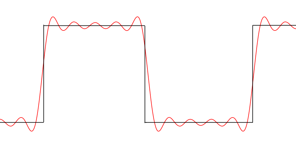
One difficult aspect of filter design is that we often must not just consider the filter’s frequency domain representation, but we also must consider the effect that its spatial domain representation will have on the reconstructed signal. In particular, we must be careful with filters that have negative lobes, such as the sinc filter. Such filters can produce an effect known as ringing when applied to sharp discontinuities, where the reconstructed signal oscillates about the signal being sampled. Take a look at the plot of a square wave being reconstructed with a sinc filter:
Key Takeaway Points:
- Error resulting from inadequate sampling rate is known as prealiasing. Error introduced through poor filtering is known as postaliasing.
- A filter’s ability to limit aliasing can be estimated by observing its frequency domain representation
- A filter’s rate of change in the spatial domain is inversely related to its rate of change in the frequency domain
- A filter’s spatial domain representation can also have an effect on the quality of the reconstructed signal, with the most notable effect being ringing occurring at discontinuities.
References
[1]http://en.wikipedia.org/wiki/Signal_processing
[2]http://en.wikipedia.org/wiki/Nyquist-Shannon_sampling_theorem
[3]Pharr, Matt and Humphreys, Greg. Physically Based Rendering - From Theory to Implementation, 2nd Edition.
[4]Akenine-Möller, Tomas, Haines, Eric, and Hoffman, Naty. Real-Time Rendering, 3rd Edition
[5]Glassner, Andrew. Principles of Digital Image Synthesis
Next article in the series:
Applying Sampling Theory To Real-Time Graphics
Comments:
MJP -
@AmazingFactory - yes you are correct, the Nyquist rate is equal to 2 times the *baseband* bandwidth, where baseband bandwidth is equal to the maximum frequency. I actually described passband bandwidth which is MaxFrequency - MinFrequency, which isn’t what you’re interested in for determining Nyquist rate. I updated the text to be more clear on this. Thank you for pointing that out!
#### [AmazingFactory]( "first10@btinternet.com") -
Aha! If the texture has a high frequency periodic pattern then you will get a moire pattern - which is an alias Also you can see why the sampling frequency must be GREATER than 2x the highest frequency Imagine sampling a 1 Hz sine wave at 2 Hz … the resulting signal could be zero (depending on the phase)
#### [Jeremy Shopf » Image Reconstruction and MSAA](http://jshopf.com/blog/?p=304 "") -
[…] with Reconstruction Filters for MSAA Resolve”. Even better, he had previously posted a nice sampling theory primer and introduction to MSAA which were also well done. Anti-aliasing was something that was really […]
#### [Ryan Monroe]( "monroe@jpl.nasa.gov") -
@AmazingFactory, @MJP Actually, I believe that it’s a bit more complicated than that. In an ideal scenario, you can just sample at twice the passband bandwidth, but if that passband is ill-located, you could need more bandwidth to represent it. Remember that signals alias/fold down when under-sampled. So, if you had a signal at, say, 25-75 Hz and were sampling at 100 Hz (twice the bandwidth), you’d see the 75->50 Hz component folding back on the 25 -> 50 Hz component (note the order of the first component, this is intentional). Then, the 0 -> 25 Hz component would still have no signal (being outside the passband and not seeing any components) and the 25->50 component would contain the mixed-up information of the entire 50 Hz of spectral data. You would have to downconvert the signal to baseband, convert it to an analytic signal or something to be able to use that spectrum efficiently. I hope this has been descriptive! Oh the banes of posting after a glass of wine ;-)
#### [Alexander](http://jstroot23.bravejournal.com/entry/128165/ "alexander_peacock@arcor.de") -
I’m not sure where you are getting your information, but good topic. I needs to spend some time learning more or understanding more. Thanks for magnificent info I was looking for this info for my mission.
#### [MJP](http://mynameismjp.wordpress.com/ "mpettineo@gmail.com") -
Thank you Andy, I’m glad that you found the article useful! That was indeed a typo, thank you for pointing that out.
#### [Andy Southwell](http://www.indygamedev.com "andy@indygamedev.com") -
Fantastic article - thank you very much! So many articles on this kind of subject go totally crazy on the maths, leaving mere mortals like me behind. One really minor typo in the final ’take away points’ : “A filter’s ability to limit aliasing can estimating by observing”. I’m guessing ’estimating’ should be ’estimate’? Anyway, keep up the good work - thanks again!
#### [Series of articles on anti-aliasing | Light is beautiful](http://lousodrome.net/blog/light/2012/10/29/series-of-articles-on-anti-aliasing/ "") -
[…] Signal Processing Primer […]
#### [MJP](http://mynameismjp.wordpress.com/ "mpettineo@gmail.com") -
Hey Rim, how’s it going? Sorry for taking so long to reply. Texture filtering is a sampling/reconstruction process, so it definitely qualifies as a convolution! I didn’t mention it because I talk about texture filtering more in-depth in the next article. As for the copies, usually it’s explained as occuring due to the properties of the shah function (impulse train). Basically the fourier transform a shah function is another shah function with the inverse period. So if you think of discrete sampling as multiplying a continuous function with a shah function with period equal to your sampling rate, this would mean that you’re convolving the frequency-domain representation of that function with a shah function with inverse period (since multiplication in the spatial/time domain is convolution in the frequency domain and vice versa). The “inverse period” bit is then what leads to the copies being closer together for lower sampling rates. There’s a pretty good explanation in Physically Based Rendering if you have that, and it’s also mentioned in Principles of Digital Image Synthesis (which is free to download). I suppose that’s true regarding information in the frequency domain. I tend to only look at these things from a graphics POV. :P Personally all of the material I’ve read has only brought up overshoot in the context of ringing. But if your book talks about it separately than I’m sure it’s a worthy topic on its own. There’s so much I haven’t read yet!
#### [oh]( "oren.hazi@gmail.com") -
When you’re sampling data for storage in memory, you’re not only sampling the signal at a particular instant, you’re also discretizing it to fit into your sample slot. For example, 8-bit sampling gives you 256 “levels” for representing the signal value, so you won’t be able to detect small differences in your signal amplitude as well as you could with a 16-bit sampler. If you make certain (reasonable, in some cases) assumptions about your input signal, you can treat the quantization distortion as a stochastic process and actually make useful statements about what this does to your spectrum, and how much headroom you need in various places to do whatever it was you wanted to do with your sampled signal. Not exactly “introductory” material, but useful when trying to answer questions like “how many bits should my analog to digital converter have?”
#### [Robin Green]( "robin.green@gmail.com") -
My favorite factoid about sampling: The trade-off between Spatial and Spectral Compactness is exactly Heisenberg’s Uncertainty Principal.
#### [AmazingFactory]( "first10@btinternet.com") -
Very enjoyable reading I think Nyquist must be greater than double the highest frequency, not double the bandwidth So to sample audio up to 22khz you need a sampling frequency greater than 44 khz (eg 44.1khz) You can not “perfectly reconstruct a signal” (unless by chance it happened to be an ideal signal)
#### [Rim]( "remigius@netforge.nl") -
As it happens, I was just reading up on DSP, so I’ll chip in. Thanks for the post at any rate, your treatise gives the more theoretical book I’m reading some more flavour. I realize I don’t have anything really valuable to add, just some ramblings relating your stuff to the book. “Working with discrete samples has a lot of advantages.” - My DSP book points out the subtlety that discrete samples are the only way to do digital signal processing in the first place. Continuous functions can’t be represented by digital equipment. It may sound puritan, but I found it to be a valuable insight. “If you’ve ever written a full-screen Gaussian blur shader, then you’ve used convolution.” - Wouldn’t linear texture filtering (non-point at any rate) already classify as convolution? It’s a simple kernel and it’s mostly used implicitly to be sure, but I think more folks could relate to that. “When this signal is discretely sampled, an infinite number of “copies” of the signal will appear…” - My book spent numerous chapters on why this occurs and I’d still be hesitant to say whether this is an artefact from the way computers have to represent signals (periodic discrete, right?) or something more fundamental. Can you share your insight on this? “Nyqust rate is … the minimum sampling rate required to perfectly reconstruct a signal without aliasing” - My book makes a big point about this being the theoretical minimum. The cut-off for bandlimiting, your stopband, won’t be perfect (it’s always a tradeoff IIRC) so it’s a good idea to err on the safe side, ie to use a higher rate. “The field of filter design is primarily concerned with this process of analyzing a filter’s frequency domain spectrum, and using that to evaluate or approximate that filter’s overall performance.” - That’d depend on whether your signal’s information is encoded in the frequency domain or the time/spatial domain ;) “Such filters can produce an effect known as ringing” - And overshoot? Two sides of the same coin, or are they as distinct as my book makes them out to be? I’m not far into filter design yet, let alone image filtering. For now, my research focusses on toying with the FFT in all its glory. If you’re interested in bouncing some ideas back and forth on this topic or DSP in general, please feel free to shoot me an e-mail.
#### [Niels Fröhling (@Ethatron)](http://twitter.com/Ethatron "niels@paradice-insight.us") -
I think it’s worth to mention that the theory still works in the analogue sample domain, that is with sample-points of infinite precision. I expect you’ll get to quantization in a later article (with lovely blue sky-pics that have banding even with floating-point render-targets :^D).
#### []( "") -
Ryan - check out the difference between baseband and passband in the MJP posts above - it’s always the baseband, or maximum frequency, that determines the Nyquist value. So if you are sampling a signal that is 74-75 Hz, the Nyquist is 150 Hz, not 2 Hz.
#### [Ryan Monroe]( "monroe@jpl.nasa.gov") -
yeah, but in that case, you *could* sample at 2 Hz. You’d then be operating in what’s known as (in that case) the 75th nyquist zone. You would be able to reproduce the original signal exactly by knowing which frequency band it originated from.
#### [AmazingFactory]( "first10@btinternet.com") -
I still can’t see why aliasing (ghosts/clones) is relevant to computer graphics. We don’t perform fourier transforms, so those clones are not an issue … Also we never sample light amplitudes to determine frequency textures are arrays of weights per channel/frequency (red, green or blue) So whilst you can consider a texture as “a signal” the frequency information is of no interest to us
#### [#3 Audio Programming Tutorial: Understanding Digital Audio | Nikkies Tutorials](https://nikkiestutorials.com/2015/01/07/3-audio-programming-tutorial-understanding-digital-audio/ "") -
[…] More information on sampling (written with graphics in mind, but the same concepts apply to digital audio): http://mynameismjp.wordpress.com/2012/10/15/signal-processing-primer/ […]
