Applying Sampling Theory To Real-Time Graphics
Previous article in the series: Signal Processing Primer
Computer graphics is a field that constantly deals with discrete sampling and reconstruction of signals, although you might not be aware of it yet. This article focuses on the ways in which sampling theory can be applied to some of the common tasks routinely performed in graphics and 3D rendering.
Image Scaling
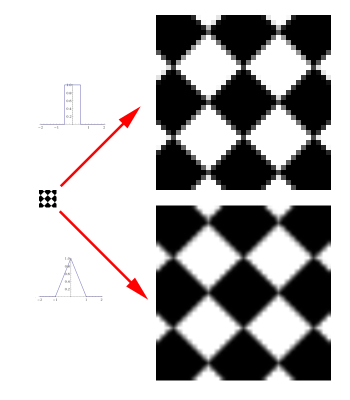
The concepts of sampling theory can are most easily applicable to graphics in the form of image scaling. An image, or bitmap, is typically the result of sampling a color signal at discrete XY sample points (pixels) that are evenly distributed on a 2D grid. To rescale it to a different number of pixels, we need to calculate a new color value at sample points that are different from the original pixel locations. In the previous article we mentioned that this process is known as resampling, and is also referred to as interpolation. Any graphics programmer should be familiar with the point (also known as nearest-neighbor) and linear (also known as bilinear) interpolation modes supported natively in GPU’s which are used when sampling textures. In case you’re not familiar, point filtering simply picks the closest texel to the sample point and uses that value. Bilinear filtering on the other hand picks the 4 closest texels, and linearly interpolates those values in the X and Y directions based on the location of the sample point relative to the texels. It turns out that these modes are both just implementations of a reconstruction filter, with point interpolation using a box function and linear interpolation using a triangle function. If you look back at the diagrams showing reconstruction with a box function and triangle function, you can see actually see how the reconstructed signal resembles the visual result that you get when performing point and linear sampling. With the box function you end up getting a reconstructed value that’s “snapped” to the nearest original sample point, while with a triangle function you end up with straight lines connecting the sample points. If you’ve used point and linear filtering, you probably also intuitively understand that point filtering inherently results in more aliasing than linear filtering when resizing an image. For reference, here’s an image showing the same rotated checkerboard pattern being resampled with a box filter and a triangle filter:
Knowing what we do about aliasing and reconstruction filters, we can now put some mathematical foundation behind what we intuitively knew all along. The box function’s frequency domain equivalent (the sinc function) is smoother and wider than the triangle function’s frequency domain equivalent (the sinc2 function), which results in significantly more postaliasing. Of course we should note even though the triangle function might be considered among the the “low end” of reconstruction filters in terms of quality, it is still attractive due to its low performance impact. Not only is the triangle function very cheap to evaluate at a given point in terms of ALU instructions, but more importantly the function evaluates to 0 for all distances greater than or equal to 1. This is important for performance, because it means that any pixels that are further than a distance of 1.0 from the resampled pixel location will not have to be considered. Ultimately this means that we only need to fetch a maximum of 4 pixels (in a 2x2 area) for linear filtering, which limits bandwidth usage and cache misses. For point filtering the situation is even better, since the box function hits zero at 0.5 (it has a width of 1.0) and thus we only need to fetch one pixel.
Outside of realtime 3D rendering, it is common to use cubic filters (also known as bicubic filters) as a higher-quality alternative to point and linear filters when scaling images. A cubic filter is not a single filtering function, but rather a family of filters that interpolate using a 3rd-order (cubic) polynomial. The use of such functions in image processing dates back to Hsieh Hou’s paper entitled “Cubic Splines for Image Interpolation and Digital Filtering”[1] which proposed using cubic B-splines as the basis for interpolation. Cubic splines are attractive for filtering because they can be used to create functions where the 1st derivative is continuous across the entire domain range, which known as being C1 continuous. Being C1 continuous also implies that the function is C0 continuous, which means that the 0th derivative is also continuous. So in other words, the function itself will would have no visible discontinuities if you were to plot the function. Remember that there is an inverse relationship between rate of change in the spatial domain and the frequency domain, therefore a smooth function without discontinuities is desirable for reducing postaliasing. A second reason that cubic splines are attractive is that the functions can be made to be zero-valued after a certain point, much like a box or triangle function. This means the filter will have a limited width, which is optimal from a performance point of view. Typically cubic filters use functions defined along the [-2, 2] range, which is double the width of a unit triangle function. Finally, a third reason for the attractiveness of cubic filters is that they can be made to produce acceptable results when applied as a seperable filter. Seperable filters can be applied independently in two passes along the X and Y dimensions, which reduces the number of neighboring pixels that need to be considered when applying the filter and thus improves the performance.
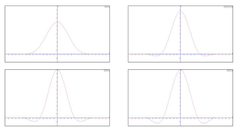
In 1988, Don Mitchell and Arun Netravali published a paper entitled Reconstruction Filters in Computer Graphics[2] which narrowed down the set of possible of cubic filtering functions into a generalized form dependent on two parameters called B and C. This family of functions produces filtering functions that are always C1 continuous, and are normalized such that area under the curve is equal to one. The general form they devised is found below:
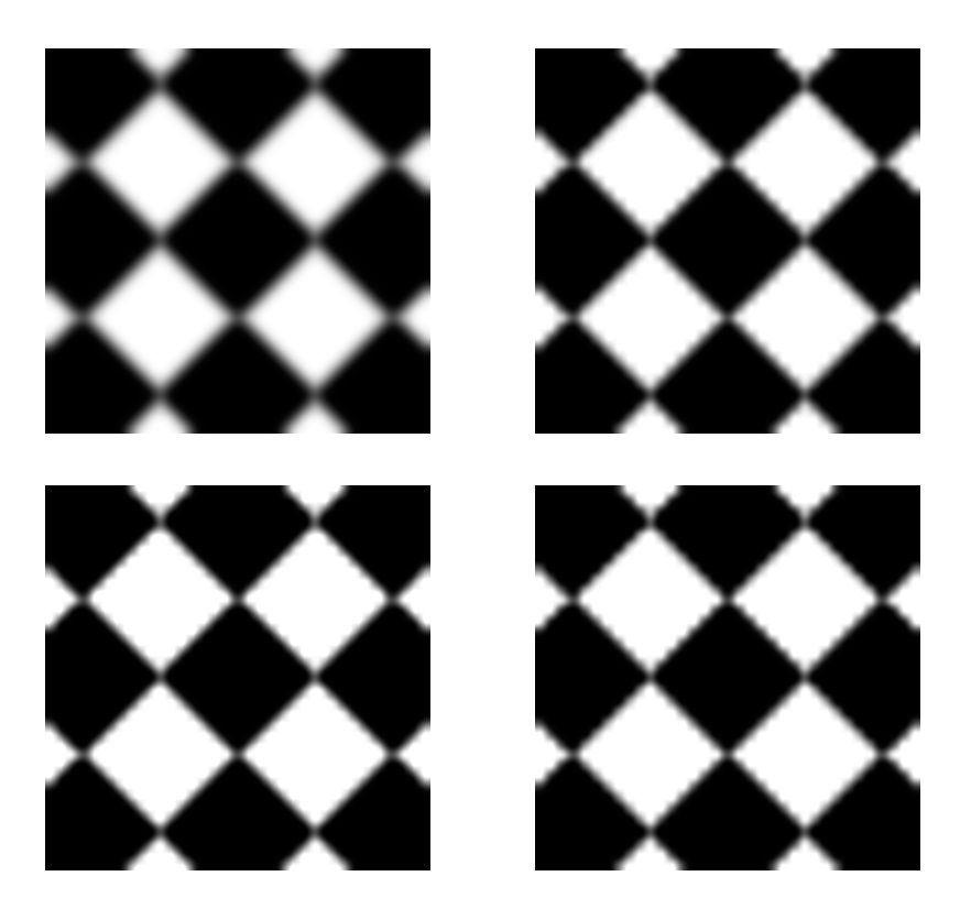
Below you can find graphs of some of the common curves in use by popular image processing software[3], as well as the result of using them to enlarge the rotated checkerboard pattern that we used earlier:
One critical point touched upon in Mitchell’s paper is that the sinc function isn’t usually desirable for image scaling, since by nature the pixel structure of an image leads to discontinuities which results in unbounded frequencies. Therefore ideal reconstruction isn’t possible, and ringing artifacts will occur due to Gibb’s phenomenon. Ringing was identified by Schrieber and Troxel[4] as being one of four negative artifacts that can occur when using cubic filters, with the other three being aliasing, blurring and anisotropy effects. Blurring is recognized as the loss of detail due to too much attenuation of higher frequencies, and is often caused by a filter kernel that is too wide. Anisotropic effects are artifacts that occur due to applying the function as a separable filter, where the resulting 2D filtering function doesn’t end up being radially symmetrical.
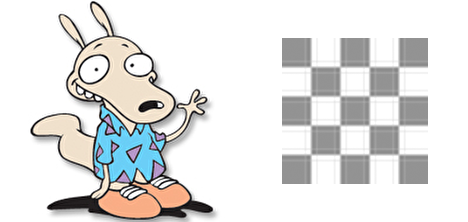
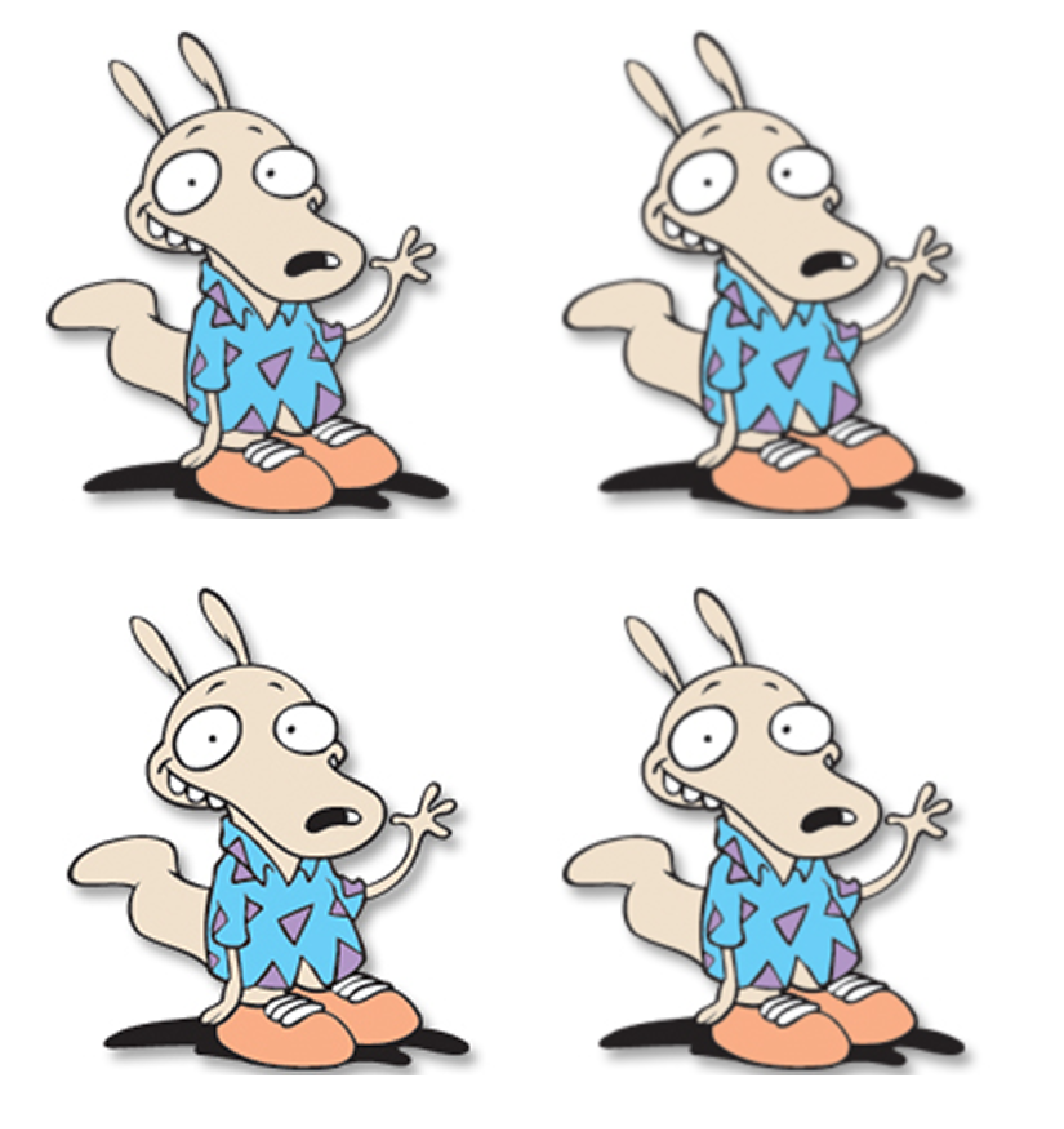
Mitchell suggested that the purely frequency domain-focused techniques of filter design were insufficient for designing a filter that produces subjectively pleasing results to the human eye, and instead emphasized balancing the 4 previously-mentioned artifacts against the amount of postaliasing in order to design a high-quality filter for image scaling. He also suggested studying human perceptual response to certain artifacts in order to subjectively determine how objectionable they may be. For instance, Earl Brown[5] discovered that ringing from a single negative lobe can actually increase perceived sharpness in an image, and thus can be a desirable effect in certain scenarios. He also pointed out that ringing from multiple negative lobes, such as what you get from a sinc function, will always degrade quality. Here’s an image of our friend Rocko enlarged with a Sinc filter, as well as an image of a checkerboard pattern enlarged with the same filter:
Ultimately, Mitchell segmented the domain of his B and C parameters into what he called “regions of dominant subjective behavior. In other words, he determined which values of each parameter resulted in undesirable artifacts. In his paper he included the following chart showing which artifacts were associated with certain ranges of the B and C parameters:
Based on his analysis, Mitchell determined that (1/3, 1/3) produced the highest-quality results. For that reason, it is common to refer to the resulting function as a “Mitchell filter”. The following images show the results of using non-ideal parameters to enlarge Rocko, as well as the results from using Mitchell’s suggested parameters:
Texture Mapping
Real-time 3D rendering via rasterization brings about its own particular issues related to aliasing, as well as specialized solutions for dealing with them. One such issue is aliasing resulting from resampling textures at runtime in order to map them to a triangle’s 2D projection in screen space, which I’ll refer to as texture aliasing. If we take the case of a 2D texture mapped to a quad that is perfectly perpendicular to the camera, texture sampling essentially boils down to a classic image scaling problem: we have a texture with some width and height, the quad is scaled to cover a grid of screen pixels with a different width and height, and the image must be resampled at the pixel locations where pixel shading occurs. We already mentioned in the previous section that 3D hardware is natively capable of applying “linear” filtering with a triangle function. Such filtering is sufficient for avoiding severe aliasing artifacts when upscaling or downscaling, although for downscaling this only holds true when downscaling by a factor <= 2.0. Linear filtering will also prevent aliasing when rotating an image, which is important in the context of 3D graphics since geometry will often be rotated arbitrarily relative to the camera. Like image scaling, rotation is really just a resampling problem and thus the same principles apply. The following image shows how the pixel shader sampling rate changes for a triangle as it’s scaled and rotated:
Mipmapping
When downscaling by a factor greater than 2, linear filtering leads to aliasing artifacts due to high-frequency components of the source image leaking into the downsampled version. This manifests as temporal artifacts, where the contents of the texture appear to flicker as a triangle moves relative to the camera. This problem is commonly dealt with in image processing by widening the filter kernel so that its width is equal to the size of the downscaled pixel. So for instance if downscaling from 100x100 to 25x25, the filter kernel would be greater than or equal in width to a 4x4 square of pixels in the original image. Unfortunately widening the filter kernel isn’t usually a suitable option for realtime rendering, since the number of memory accesses increases with O(N2) as the filter width increases. Because of this a technique known as mipmapping is used instead. As any graphics programmer should already know, mipmaps consist of a series of prefiltered versions of a 2D texture that were downsampled with a kernel that’s sufficiently wide enough to prevent aliasing. Typically these downsampled versions are generated for dimensions that are powers of two, so that each successive mipmap is half the width and height of the previous mipmap. The following image from Wikipedia shows an example of typical mipmap chain for a texture:
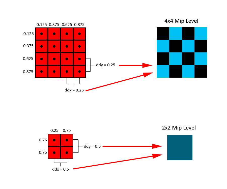
A box function is commonly used for generating mip maps, although it’s possible to use any suitable reconstruction filter when downscaling the source image. The generation is also commonly implemented recursively, so that each mip level is generated from the mip level preceding it. This makes the process computationally cheap, since a simple linear filter can be used at each stage in order to achieve the same results as a wide box filter applied to the highest-resolution image. At runtime the pixel shader selects the appropriate mip level by calculating the gradients of the texture coordinate used for sampling, which it does by comparing texture coordinate used for one pixel to the texture coordinate used in the neighboring pixels of a 2x2 quad. These gradients, which are equal to the partial derivatives of the texture coordinates with respect to X and Y in screen space, are important because they tell us the relationship between a given 2D image and the rate at which we’ll sample that image in screen space. Smaller gradients mean that the sample points are close together, and thus we’re using a high sampling rate. Larger gradients result from the sample points being further apart, which we can interpret to mean that we’re using a low sampling rate. By examining these gradients we can calculate the highest-resolution mip level that would provide us with an image size less than or equal to our sampling rate. The following image shows a simple example of mip selection:
In the image, the two red rectangles represent texture-mapped quads of different sizes rasterized to a 2D grid of pixels_._ For the topmost quad, the a value of 0.25 will be computed as the partial derivative for the U texture coordinate with respect to the X dimension, and the same value will be computed as the partial derivative for the V texture coordinate with respect to the Y dimension. The larger of the two gradients is then used to select the appropriate mip level based on the size of the texture. In this case, the length of the gradient will be 0.25 which means that the 0th (4x4) mip level will be selected. For the lower quad the size of the gradient is doubled, which means that the 1st mip level will be selected instead. Quality can be further improved through the use of trilinear filtering, which linearly interpolates between the results of bilinearly sampling the two closest mip levels based on the gradients. Doing so prevents visible seams on a surface at the points where a texture switches to the next mip level.
One problem that we run into with mipmapping is when an image needs to be downscaled more in one dimension than in the other. This situation is referred to as anisotropy, due to the differing sampling rates with respect to the U and V axes of the texture. This happens all of the time in 3D rendering, particularly when a texture is mapped to a ground plane that’s nearly parallel with the view direction. In such a case the plane will be projected such that the V gradients grow more quickly than the U gradients as distance from the camera increases, which equates to the sampling rate being lower along the V axis. When the gradient is larger for one axis than the other, 3D hardware will use the larger gradient for mip selection since using the smaller gradient would result in aliasing due to undersampling. However this has the undesired effect of over-filtering along the other axis, thus producing a “blurry” result that’s missing details. To help alleviate this problem, graphics hardware supports anisotropic filtering. When this mode is active, the hardware will take up to a certain number of “extra” texture samples along the axis with the larger gradient. This allows the hardware to “reduce” the maximum gradient, and thus use a higher-resolution mip level. The final result is equivalent to using a rectangular reconstruction filter in 2D space as opposed to a box filter. Visually such a filter will produce results such that aliasing is prevented, while details are still perceptible. The following images demonstrate anisotropic filtering on a textured plane:
Geometric Aliasing
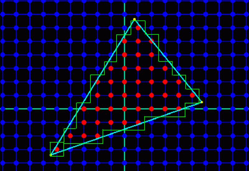
A second type of aliasing experienced in 3D rendering is known as geometric aliasing. When a 3D scene composed of triangles is rasterized, the visibility of those triangles is sampled at discrete locations typically located at the center of the screen pixels. Triangle visibility is just like any other signal in that there will be aliasing in the reconstructed signal when the sampling rate is inadequate (in this case the sampling rate is determined by the screen resolution). Unfortunately triangular data will always have discontinuities, which means the signal will never be bandlimited and thus no sampling rate can be high enough to prevent aliasing. In practice these artifacts manifest as the familiar jagged lines or “jaggies” commonly seen in games and other applications employing realtime graphics. The following image demonstrates how these aliasing artifacts occur from rasterizing a single triangle:
Although we’ve already established that no sampling rate would allow us to perfectly reconstruct triangle visibility, it is possible to reduce aliasing artifacts with a process known as oversampling. Oversampling essentially boils down to sampling a signal at some rate higher than our intended output, and then using those samples points to reconstruct new sample points at the target sampling rate. In terms of 3D rendering this equates to rendering at some resolution higher than the output resolution, and then downscaling the resulting image to the display size. This process is known as supersampling, and it’s been in use in 3D graphics for a very long time. Unfortunately it’s an expensive option, since it requires not just rasterizing at a higher resolution but also shading pixels at a higher rate. Because of this, an optimized form of supersampling known as multi-sample antialiasing (abbreviated as MSAA) was developed specifically for combating geometric aliasing. We’ll discuss MSAA and geometric aliasing in more detail in the following article.
Shader Aliasing
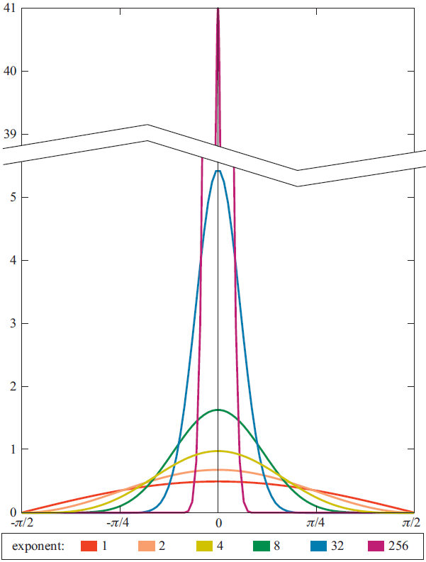
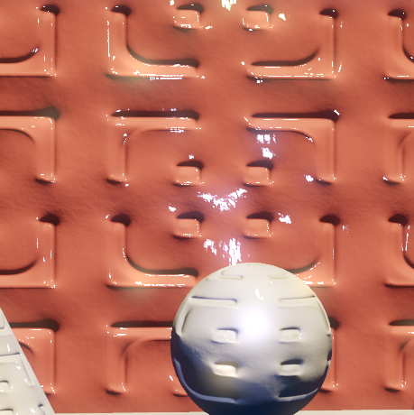
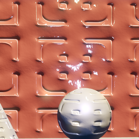
A third type of aliasing that’s common in modern 3D graphics is known as shader aliasing. Shader aliasing is similar to texture aliasing, in that occurs due to the fact that the pixel shader sampling rate is fixed in screen space. However the distinction is that shader aliasing refers to undersampling of signals that are evaluated analytically in the pixel shader using mathematical formulas, as opposed to undersampling of a texture map. The most common and noticeable case of shader aliasing results from applying per-pixel specular lighting with low roughness values (high specular exponents for Phong and Blinn-Phong). Lower roughness values result in narrower lobes, which make the specular response into a higher-frequency signal and thus more prone to undersampling. The following image contains plots of the N dot H response of a Blinn-Phong BRDF with varying roughness, demonstrating it becomes higher frequency for lower roughnesses:
Shader aliasing is most likely to occur when normal maps are used, since they increase the frequency of the surface normal and consequently cause the specular response to vary rapidly across a surface. HDR rendering and physically-based shading models can compound the problem even further, since they allow for extremely intense specular highlights relative to the diffuse lighting response. This category of aliasing is perhaps the most difficult to solve, and as of yet there are no silver-bullet solutions. MSAA is almost entirely ineffective, since the pixel shading rate is not increased compared to the non-MSAA. Supersampling is effective, but prohibitively expensive due to the increased shader and bandwidth costs required to shade and fill a larger render target. Emil Persson demonstrated a method of selectively supersampling the specular lighting inside the pixel shader[6], but this too can be expensive if the number of lights are high or if multiple normal maps need to be blended in order to compute the final surface normal.
A potential solution that has been steadily gaining some ground[7][8] is to modify the specular shading function itself based on normal variation. The theory behind this is that microfacet BRDF’s naturally represent micro-level variation along a surface, with the amount of variation being based on a roughness parameter. If we increase the roughness of a material as the normal map details become relatively smaller in screen space, we use the BRDF itself to account for the undersampling of the normal map/specular lighting response. Increasing roughness decreases the frequency of the resulting reflectance, which in turn reduces the appearance of artifacts. The following image contains an example of using this technique, with an image captured with 4x shader supersampling as a reference:
This approach (and others like it) can be considered to be part of a broader category of antialiasing techniques known as prefiltering. Prefiltering amounts to applying some sort of low-pass filter to a signal before sampling it, with the goal of ensuring that the signal’s bandwidth is less than half of the sampling rate. In a lot of cases this isn’t practical for graphics since we don’t have adequate information about what we’re sampling (for instance, we don’t know what triangle should is visible for a pixel until we sample and raterize the triangle). However in the case of specular aliasing from normal maps, the normal map contents are known ahead of time.
Temporal Aliasing
So far, we have discussed graphics in terms of sampling a 2D signal. However we’re often concerned with a third dimension, which is time. Whenever we’re rendering a video stream we’re also sampling in the time domain, since the signal will completely change as time advances. Therefore we must consider sampling along this dimension as well, and how it can produce aliasing.
In the case of video we are still using discrete samples, where each sample is a complete 2D image representing our scene at some period of time. This sampling is similar to our sampling in the spatial domain: there is some frequency of the signal we are sampling, and if we undersample that signal aliasing will occur. One classic example of a temporal aliasing is the so-called “wagon-wheel effect”, which refers to the phenomenon where a rotating wheel may appear to rotate more slowly (or even backwards) when viewed in an undersampled video stream. This animated GIF from Wikipedia demonstrates the effect quite nicely:
In games, temporal sampling artifacts usually manifest as “jerky” movements and animations. Increases in framerate correspond to an increase in sampling rate along the time domain, which allows for better sampling of faster-moving content. This is directly analogous to the improvements that are visible from increasing output resolution: more details are visible, and less aliasing is perceptible.
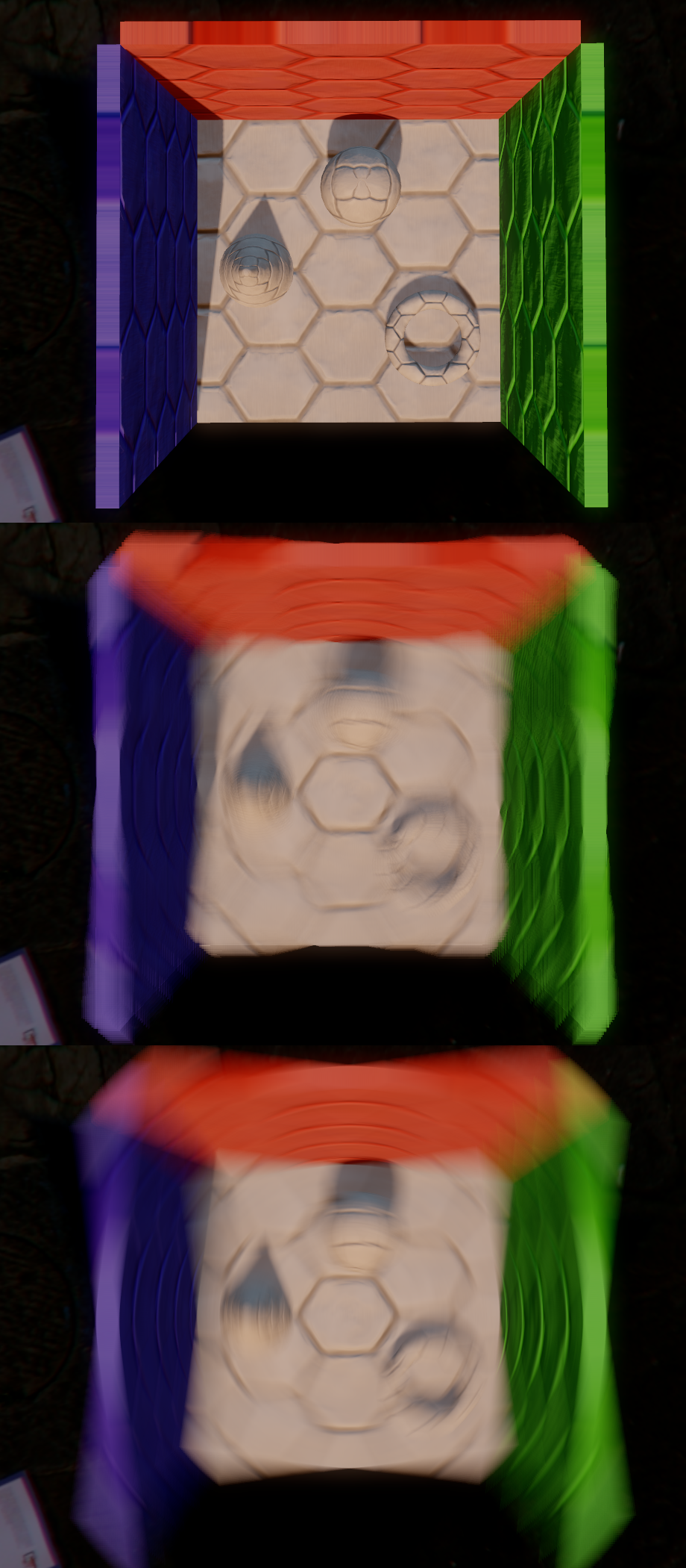
The most commonly-used anti-aliasing technique for temporal aliasing is motion blur. Motion blur actually refers to an effect visible in photography, which occurs due to the shutter of the camera being open for some non-zero amount of time. This produces a result quite different than what we produce in 3D rendering, where by default we get an image representing one infinitely-small period of time. To accurately simulate the effect, we could supersample in the time domain by rendering more frames than we output and applying a filter to the result. However this is prohibitively expensive just like spatial supersampling, and so approximations are used. The most common approach is to produce a per-pixel velocity buffer for the current frame, and then use that to approximate the result of oversampling with a blur that uses multiple texture samples from nearby pixels. Such an approach can be considered an example of advanced reconstruction filter that uses information about the rate of change of a signal rather than additional samples in order to reconstruct an approximation of the original sample. Under certain conditions the results can be quite plausible, however in many cases noticeable artifacts can occur due to the lack of additional sample points. Most notably these artifacts will occur where the occlusion of a surface by another surface changes during a frame, since information about the occluded surface is typically not available to the post-process shader performing the reconstruction. The following image shows three screenshots of a model rotating about the camera’s z-axis: the model rendered with no motion blur, the model rendered with Morgan McGuire’s post-process motion blur technique[9] applied using 16 samples per pixel, and finally the model rendered temporal supersampling enabled using 32 samples per frame”
References
[1] Hou, Hsei. Cubic Splines for Image Interpolation and Digital Filtering. IEEE Transactions on Acoustics, Speech, and Signal Processing. Vol. 26, Issue 6. December 1978.
[2] Mitchell, Don P. and Netravali, Arun N. Reconstruction Filters in Computer Graphics. SIGGRAPH ‘88 Proceedings of the 15th annual conference on Computer graphics and interactive techniques.
[3] http://entropymine.com/imageworsener/bicubic/
[4] Schreiber, William F. Transformation Between Continuous and Discrete Representations of Images: A Perceptual Approach. IEEE Transactions on Pattern Analysis and Machine Intelligence. Volume 7, Issue 2. March 1985.
[5] Brown, Earl F. Television: The Subjective Effects of Filter Ringing Transients. February, 1979.
[6] http://www.humus.name/index.php?page=3D&ID=64
[7] http://blog.selfshadow.com/2011/07/22/specular-showdown/
[8] http://advances.realtimerendering.com/s2012/index.html
[9] McGuire, Morgan. Hennessy, Padraic. Bukowski, Michael, and Osman, Brian. A Reconstruction Filter for Plausible Motion Blur. I3D 2012.
Next article in the series: A Quick Overview of MSAA
Comments:
> In the animation the camera is moving to the right at a constant speed Actually, that’s not true. According to the wikipedia description of the gif, it’s the acceleration that’s constant, not the speed. (Which makes much more sense!)
#### [Ruud van Gaal](http://www.racer.nl "ruud@racer.nl") -
Interesting article; now onto learning more on frequency lowering for specular highlights, which is indeed a problem (well, I have several areas of shimmering in my graphics engine).
#### [AmazingFactory]( "first10@btinternet.com") -
worth mentioning that cubic b-spline interpolation results in color shift because it does not interpolate exactly also b-splines are C2 continuous (which means you can use b-spline to interpolate a heightmap and create perfectly smooth normals)
#### [Rim]( "remigius@netforge.nl") -
Interesting as usual. I’ll spare you my usual puritan amateur comments ;)
