Mitsuba Quick-Start Guide
Angelo Pesce’s recent blog post brought up a great point towards the end of the article: having a “ground-truth” for comparison can be extremely important for evaluating your real-time techniques. For approximations like pre-integrated environment maps it can help visualize what kind of effect your approximation errors will have on a final rendered image, and and in many other cases it can aid you in tracking down bugs in your implementation. On Twitter I advocated writing your own path tracer for such purposes, primarily because doing so can be an extremely educational experience. However not everyone has time to write their own path tracer, and then populate with all of the required functionality. And even if you do have the time, it’s helpful to have a “ground truth for your ground truth”, so that you can make sure that you’re not making any subtle mistakes (which is quite easy to do with a path tracer!). To help in both of these situations, it’s really handy to have a battle-tested renderer at your disposal. For me, that renderer is Mitsuba.
Mitsuba is a free, open source (GPL), physically based renderer that implements a variety of material and volumetric scattering models, and also implements some of the latest and greatest integration techniques (bidirectional path tracing, photon mapping, metropolis light transport, etc.). Since it’s primarily an academic research project, it doesn’t have all of the functionality and user-friendliness that you might get out of a production renderer like Arnold. That said, it can certainly handle many (if not all) of the cases that you would want to verify for real-time rendering, and any programmer shouldn’t have too much trouble figuring out the interface and file formats once he or she spends some time reading the documentation. It also features a plugin system for integrating new functionality, which could potentially be useful if you wanted to try out a custom material model but still make use of Mitsuba’s ray-tracing/sampling/integration framework.
To help get people up and running quickly, I’ve come up with a “quick-start” guide that can show you the basics of setting up a simple scene and viewing it with the Mitsuba renderer. It’s primarily aimed at fellow real-time graphics engineers who have never used Mitsuba before, so if you belong in that category then hopefully you’ll find it helpful! The guide will walk you through how to import a scene from .obj format into Mitsuba’s internal format, and then directly manipulate Mitsuba’s XML format to modify the scene properties. Editing XML by hand is obviously not an experience that makes anyone jump for joy, but I think it’s a decent way to familiarize yourself with their format. Once you’re familiar with how Mitsuba works, you can always write your own exporter that converts from your own format.
1. Getting Mitsuba
The latest version of Mitsuba is available on this page. If you’re running a 64-bit version of Windows like me, then you can go ahead and grab the 64-bit version which contains pre-compiled binaries. There are also Mac and Linux versions if either of those is your platform of choice, however I will be using the Windows version for this guide.
Once you’ve downloaded the zip file, go ahead and extract it to a folder of your choice. Inside of the folder you should have mtsgui.exe, which is the simple GUI version of the renderer that we’ll be using for this guide. There’s also a command-line version called mitsuba.exe, should you ever have a need for that.
While you’re on the Mitsuba website, I would also recommend downloading the PDF documentation into the same folder where you extracted Mitsuba. The docs contain the full specification for Mitsuba’s XML file format, general usage information, and documentation for the plugin API.
2. Importing a Simple Scene
Now that we have Mitsuba, we can get to work on importing a simple scene into Mitsuba’s format so that we can render it. The GUI front-end is capable of importing scenes from both COLLADA (*.dae) and Wavefront OBJ (*.obj) file formats, and for this guide we’re going to import a very simple scene from an OBJ file that was authored in Maya. If you’d like to follow along on your own, then you can grab the “TestScene.obj” file from the zip file that I’ve uploaded here: https://mynameismjp.files.wordpress.com/2015/04/testscene.zip. Our scene looks like this in Maya:
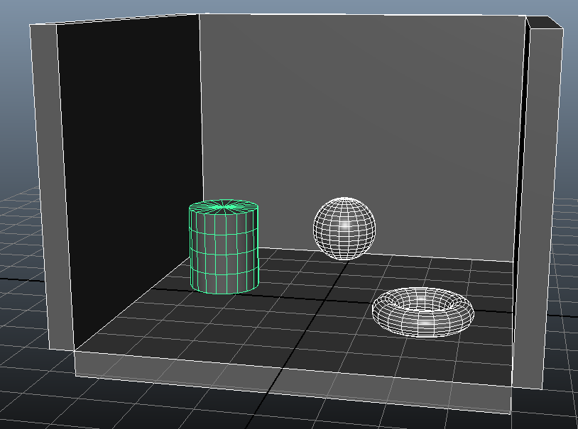
As you can see, it’s a very simple scene composed of a few primitive shapes arranged in a box-like setup. To keep things really simple with the export/import process, all of the meshes have their default shader assigned to them.
To import the scene into Mitsuba, we can now run mtsgui.exe and select File->Import from the menu bar. This will give you the following dialog:
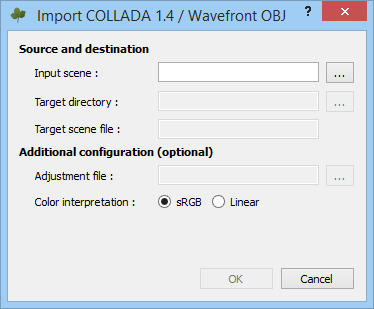
Go ahead and click the top-left button to browse for the .obj file that you’d like to import. Once you’ve done this, it will automatically fill in paths for the target directory and target file that will contain the Mitsuba scene definition. Feel free to change those if you’d like to create the files elsewhere. There’s also an option that specifies whether you’d like any material colors and textures as being in sRGB or linear color space.
Once you hit “OK” to import the scene, you should now see our scene being rendered in the viewport:
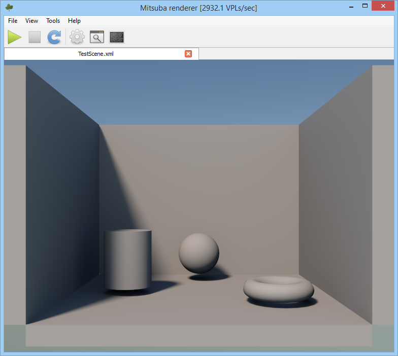
What you’re seeing right now is the OpenGL realtime preview. The preview uses the GPU to render your scene with VPL approximations for GI, so that it can give you a rough idea of what your scene will look like once it’s actually rendered. Whenever you first open a scene you will get the preview mode, and you’ll also revert back to the preview mode whenever you move the camera.
Speaking of the camera, it uses a basic “arcball” system that’s pretty similar to what Maya uses. Hold the left mouse button and drag the pointer to rotate the camera around the focus point, hold the middle mouse button to pan the camera left/right/up/down, and hold the right mouse button to move the camera along its local Z axis (you can also use the mouse wheel for this).
3. Configuring and Rendering
Now that we have our scene imported, let’s try doing an actual render. First, click the button in the toolbar with the gear icon. It should bring up the following dialog, which lets you configure your rendering settings:
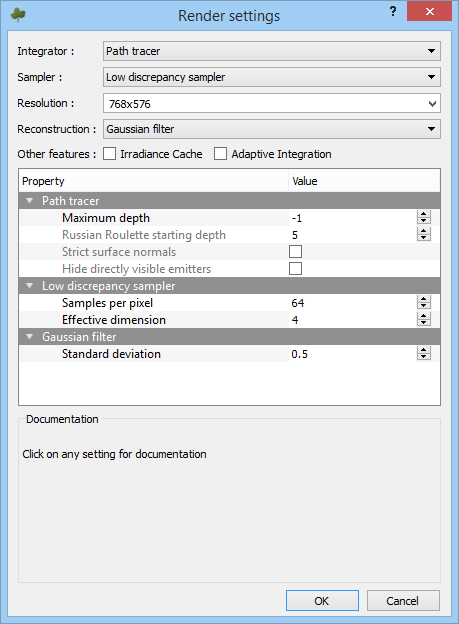
That first setting specifies which integrator that you want to use for rendering. If you’re not familiar with the terminology being used here, an"integrator" is basically the overall rendering technique used for computing how much light is reflected back towards the camera for every pixel. If you’re not sure which technique to use, the path tracer is a good default choice. It makes use of unbiased monte carlo techniques to compute diffuse and specular reflectance from both direct and indirect light sources, which essentially means that if you increase the number of samples it will always converge on the “correct” result. The main downside is that it can generate noisy results for scenes where a majority of surfaces don’t have direct visibility of emissive light sources, since the paths are always traced starting at the camera. The bidirectional path tracer aims to improve on this by also tracing additional paths starting from the light sources. The regular path tracer also won’t handle volumetrics, and so you will need to switch to the volumetric path tracer if you every want to experiment with that.
For a path tracer, the primary quality setting is the “Samples per pixel” option. This dictates how many samples to take for every pixel in the output image, and so you can effectively think of it as the amount of supersampling. Increasing it will reduce aliasing from the primary rays, and also reduce the variance in the results of computing reflectance off of the surfaces. Using more samples will of course increase the rendering time as well, so use it carefully. The “Sampler” option dictates the strategy used for generating the random samples that are used for monte carlo integration, which can also have a pretty large effect on the resulting variance. I would suggest reading through Physically Based Rendering if you’d like to learn more about the various strategies, but if you’re not sure then the “low discrepancy sampler” is a good default choice. Another important option is the “maximum depth” setting, which essentially lets you limit the renderer to using a fixed number of bounces. Setting it to 1 only gives you emissive surfaces and lights (light -> camera), setting it to 2 gives you emissive + direct lighting on all surfaces (light -> surface -> camera), setting it to 3 gives you emissive + direct lighting + 1 bounce of indirect lighting (light -> surface -> surface -> camera), and so on. The default value of -1 essentially causes the renderer to keep picking paths until it hits a light source, or the transmittance back to the camera is below a particular threshold.
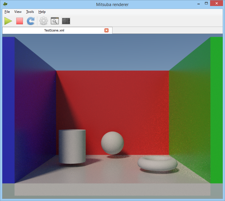
Once you’ve configured everything the way I did in the picture above, go and hit OK to close the dialog. After than, press the big green “play” button in the toolbar to start the renderer. Once it starts, you’ll see an interactive view of the renderer completing the image one tile at a time. If you have a decent CPU it shouldn’t take more than 10-15 seconds to finish, at which point you should see this:
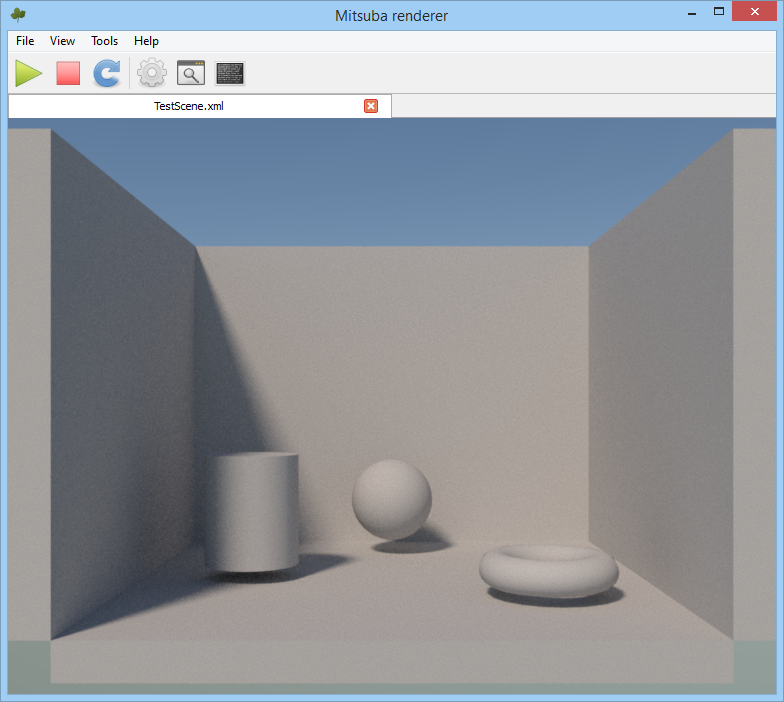
Congratulations, you now have a path-traced rendering of the scene!
4. The Scene File Format
Now that we have a basic scene rendering, it’s time to dig into the XML file for the scene and start customizing it. Go head and open up “TestScene.xml” in your favorite text editor, and have a look around. It should look like this:
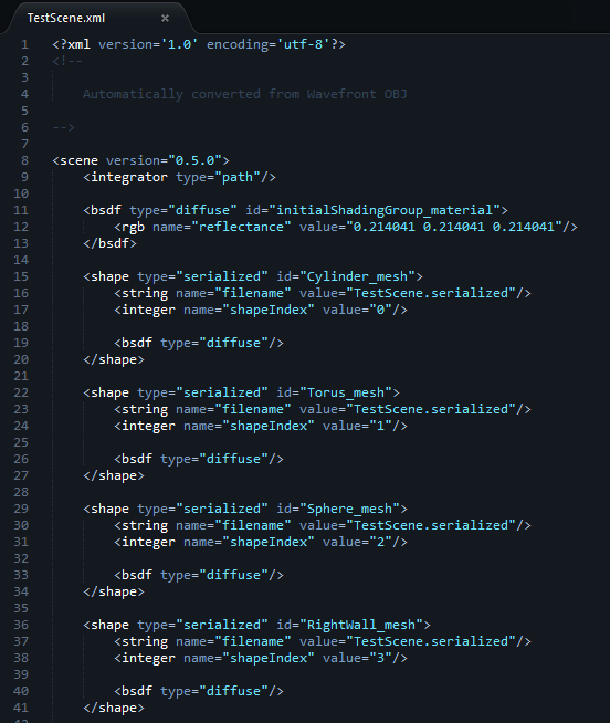
If you scroll around a bit, you’ll see declarations for various elements of the scene. Probably what you’ll notice first is a bunch of “shape” declarations: these are the various meshes that make up the scene. Since we imported from .obj, Mitsuba automatically generated a binary file called “TestScene.serialized” from our .obj file containing the actual vertex and index data for our meshes, which is then referenced by the shapes. Mitsuba can also directly reference .obj or .ply files in a shape, which is convenient if you don’t want to go through Mitsuba’s import process. It also supports hair meshes, heightfields from an image file, and various primitive shapes (sphere, box, cylinder, rectangle, and disk). Note that shapes support transform properties as well as transform hierarchies, which you can use to position your meshes within the scene as you see fit. See section 8.1 of the documentation for a full description of all of the shape types, and their various properties.
For each shape, you can see a “bsdf” property that specifies the BSDF type to use for shading the mesh. Currently all of the shapes are specifying that they should use the “diffuse” BSDF type, and that the BSDF should use default parameters. You might also notice there’s a separate bsdf declaration towards the top of the file, with an ID of “initialShadingGroup_material”. This comes from the default shader that Maya applies to all meshes, which is also reflected in the .mtl file that was generated along with the .obj file. This BSDF is not actually being used by any of the shapes in the scene, since they all are currently specifying that they just want the default “diffuse” BSDF. In the next section I’ll go over how we can create and modify materials, and then assign them to meshes.
If you scroll way down to the bottom, you’ll see the camera and sensor properties, which looks like this:
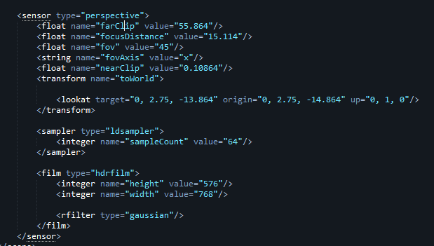
You should immediately recognize some of your standard camera properties, such as the clip planes and FOV. Here you can also see an example of a transform property, which is using the “lookAt” method for specifying the transform. Mitsuba also supports specifying transforms as translation + rotation + scale, or directly specifying the transformation matrix. See section 6.1.6 of the documentation for more details.
If you decide to manually update any of the properties in the scene, you can tell the GUI to re-load the scene from disk by clicking the button with blue, circular arrow on it in the toolbar. Just be aware that if you save the file from the GUI app, it may overwrite some of your changes. So if you decide to set up a nice camera position in the XML file, make sure that you don’t move the camera in the app and then save over it!
5. Specifying Materials
Now let’s assign some materials to our meshes, so that we can start making our scene look interesting. As we saw previously, any particular shape can specify which BSDF model it should use as well as various properties of that BSDF. Currently, all of our meshes are using the “diffuse” BSDF, which implements a simple Lambertian diffuse model. There are many BSDF types available in Mitsuba, which you can read about in section 8.2 of the documentation. To start off, we’re going to use the “roughplastic” model for a few of our meshes. This model gives you a classic diffuse + specular combination, where the diffuse is Lambertian the specular can use one of several microfacet models. It’s a good default choice for non-metals, and thus can work well for a wide variety of opaque materials. Let’s go down to about line 36 of our scene file, and make the following changes:
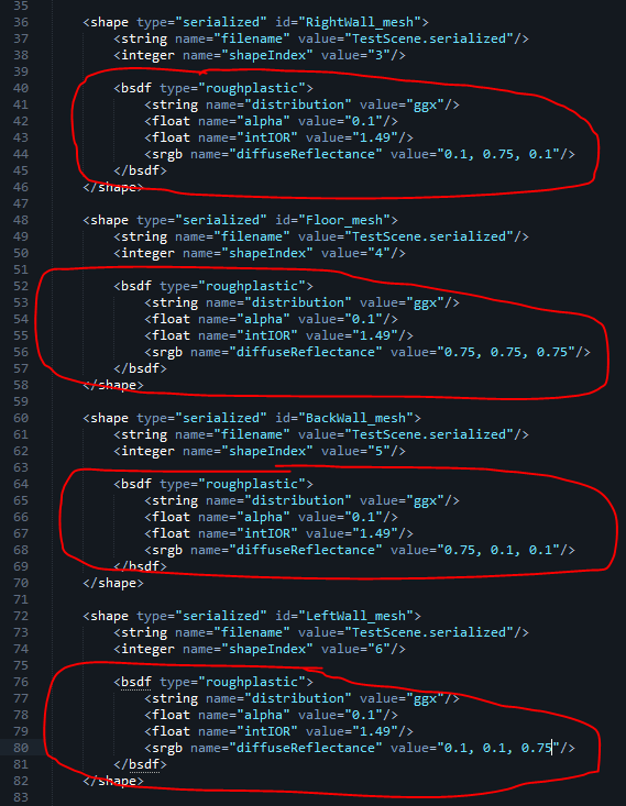
As you can see, we’ve added BSDF properties for 4 of our meshes. They’re all configured to use the “roughplastic” BSDF with a GGX distribution, a roughness of 0.1, and an IOR of 1.49. Unfortunately Mitsuba does not support specifying the F0 reflectance value for specular, and so we must specify the interior and exterior IOR instead (exterior IOR defaults to “air”, and so we can leave it at its default value). You can also see that I specified diffuse reflectance values for each shape, with a different color for each. For this I used the “srgb” property, which specifies that the color is in sRGB color space. You can also use the “rgb” property to specify linear values, or the “spectrum” property for spectral rendering.
After making these changes, go ahead click the “reload” button in Mitsuba followed by the “start” button to re-render the image. We should now get the following result:
Nice! Our results are noisier on the right side due to specular reflections from the sun, but we can now clearly see indirect specular in addition to indirect diffuse.
To simplify setting up materials and other properties, Mitsuba supports using references instead directly specifying shape properties. To see how that works, let’s delete the “initialShadingGroup_material” BSDF declaration at line 11 and replace it with a new that that we will reference into the cylinder and torus meshes:
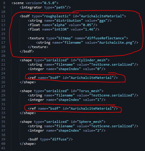
If you look closely, you’ll see that for this new material I’m also using a texture for the diffuse reflectance. When setting the “texture” property to the “bitmap” type, you can tell Mitsuba to load an image file off disk. Note that Mitsuba also supports a few built-in procedural textures that you can use, such as checkerboard and a grid. See section 8.3 for more details.
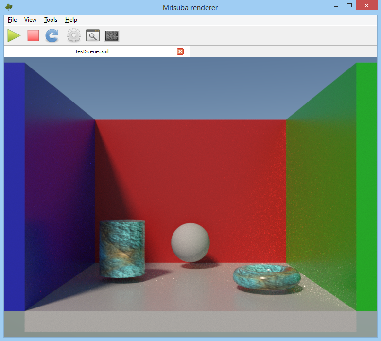
After refreshing, our render should now look like this:
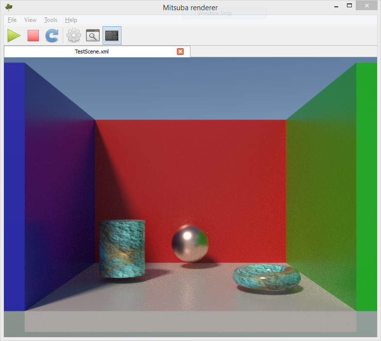
To finish up with materials, let’s assign a more interesting material to the sphere in the back:
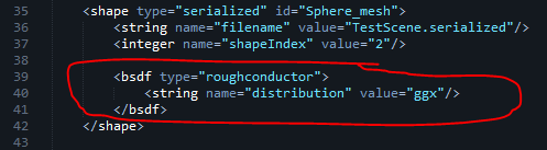
If we now re-render with a sample count of 256 to reduce the variance, we get this result:
6. Adding Emitters
Up until this point, we’ve been using Mitsuba’s default lighting environment for rendering. Mitsuba supports a variety of emitters that mostly fall into one of 3 categories: punctual lights, area lights, or environment emitters. Punctual lights are your typical point, spot, and directional lights that are considered to have an infinitesimally small area. Area lights are arbitrary meshes that uniformly emit light from their surface, and therefore must be used with a corresponding “shape” property. Environment emitters are infinitely distant sources that surround the entire scene, and can either use an HDR environment map, a procedural sun and sky model, or a constant value. For a full listing of all emitter types and their properties, consult section 8.8 of the documentation.
Now, let’s try adding an area light to our scene. Like I mentioned earlier, an area light emitter needs to be parented to a “shape” property that determines the actual 3D representation of the light source. While this shape could be an arbitrary triangle mesh if you’d like, it’s a lot easier to just use Mitsuba’s built-in primitive types instead. For our light source, we’ll use the “sphere” shape type so that we get a spherical area light source:
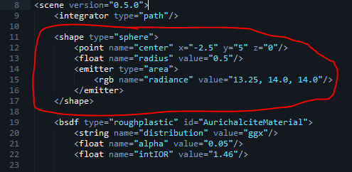
After refreshing, our scene now looks like this:
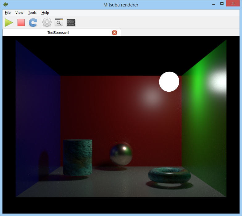
Notice how the sky and sun are now gone, since we now have an emitter defined in the scene. To replace the sky, let’s now try adding our own environment emitter that uses an environment map:
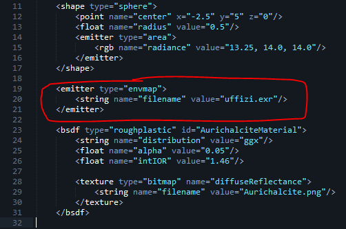
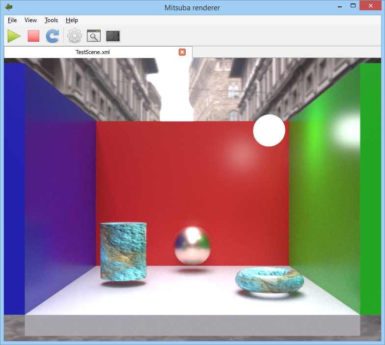
The “uffizi.exr” file used here is an HDR light probe from USC’s high-resolution image probe gallery. Note that this emitter does not support cubemaps, and instead expects a 2D image that uses equirectangular mapping. Here’s what it looks like rendered with the path tracer, using a higher sample count of 256 samples per pixel:
7. Further Reading
At this point, you should hopefully understand the basics of how to use Mitsuba, and how to set up scenes in its XML file format. There’s obviously quite a bit of functionality that I didn’t cover, which you can read about in the documentation. If you’d like to know more about how Mitsuba works, I would very strongly recommend reading through Physically Based Rendering. Mitsuba is heavily based on pbrt (which is the open-source renderer described in the book), and the book does a fantastic job of explaining all of the relevant concepts. It’s also a must-have resource if you’d like to write your own path tracer, which is something that I would highly recommend to anybody working in real-time graphics.
Oh and just in case you missed it, here’s the link to the zip file containing the example Mitsuba scene: https://mynameismjp.files.wordpress.com/2015/04/testscene.zip
Comments:
GI ground truth for comparison | How to play cool games -
[…] I’ve tried Mitsuba, as per MJP’s advice, but I really can’t get into it. It’s good, but the XML is ridiculously obtuse and […]
#### [seblagarde](http://seblagarde.wordpress.com "lagardese@hotmail.fr") -
hey, Good to see Mitsuba spreading accros game industry. We use it for frostbite too to compare our in-engine ground thruth with ground thruth :) On thing you Forgot to mention is the tone mapper. For the sake of good comparison we bypass our tone mapper in frostbite and export a screenshot in exr to compare with a exr shot produce by Mitsuba without tone mapping. Only way to have reliable result. So i think you should introduce the image postprocess control of Mitsuba too.
#### [MJP](http://mynameismjp.wordpress.com/ "mpettineo@gmail.com") -
Hi Sébastien, I agree, that’s a good topic to touch on in the tutorial. Here at RAD we also do comparisons with EXR screenshots, so that we can remove tone mapping from the mix. @Nico: I actually don’t have a lot of experience with LuxRender, so I wouldn’t be a great person to ask about that! I will definitely have to spend some time with it at some point.
#### [Nico](http://ngaloppo.wordpress.com/ "nico@crossbar.net") -
Is there any advantage of using Mitsuba vs. LuxRender? (http://www.luxrender.net/en_GB/index)
#### [Wumpf](https://twitter.com/wumpf "r_andreas2@web.de") -
Just wanted to thank you for this great introduction/tutorial! :) It helped me a lot to get started with groundtruth renderings for my realtime global illumination experiments :)
#### [Nicolas Bertoa](http://nbertoa.wordpress.com "nicolas.bertoa@outlook.com") -
Thanks for this article, Matt. You said: “It’s also a must-have resource if you’d like to write your own path tracer, which is something that I would highly recommend to anybody working in real-time graphics.” Some time ago I had the same doubt about going offline or not. Why do you think doing that will help in real-time graphics?
#### [AGraphicsGuy](http://agraphicsguy.wordpress.com "jerrycao_1985@icloud.com") -
There is an alternative by using Blender with mitsuba, which will be much simpler than the above procedure. I’m not sure if it exposes full features in mitsuba, it works pretty cool to me.
#### [Theo Gottwald](http://www.fa2.de "atg@fa2.de") -
To make Mitsuba really render specular, it needs to be compiled with a setting of spectrum(something)=30 However this specular version is nowhere to download.
#### [MJP](http://mynameismjp.wordpress.com/ "mpettineo@gmail.com") -
Hi Nicolas, I think that writing a path tracer gives you a better perspective on BRDF’s and the rendering equation, since you take a more unified approach to solving the rendering equation. In real-time we end up having to do so many specialized paths for things like point lights, area lights, environment specular, etc., since we have such strict limitations on what we can do in a single frame. Meanwhile in a path tracer you’re free to to do arbitrary queries on your scene via ray tracing, which lets you focus on integrating to solve the rendering equation. So instead of using approximation X or for one light source and technique Y for handling your environment specular, you just use ray tracing to get radiance and use the same BRDF for everything. Having that flexibility and simplicity also makes it much easier (IMO) to explore things like refraction, and volumetric scattering. This is all my own opinion based on my personal experiences, so your mileage may vary. If nothing else, knowing how a path tracer works will give you valuable knowledge for understanding how offline renderers work, or for writing an offline baking tool that you use for a real-time engine. Monte Carlo integration (which is used heavily in path tracing) is also an invaluable tool to have on your belt for almost any rendering scenario, both real-time and offline.